Indexes: B+ trees, hashing and query optimisation
Pages and access cost, B+ trees with proof of the height and an example on a billion rows, hash, primary, secondary and composite indexes, cost on writes, the optimiser and EXPLAIN.
A table with a billion rows can be read in full, but it takes minutes. Finding the customer with a given code in a few milliseconds requires an index, like that of a book. In this lesson we look at how a database organises data on disk, B+ trees with the proof of their height and a numerical example, hash indexes, composite indexes and the prefix rule, the cost of indexes on writes and the work of the optimiser.
Pages and accesses
The DBMS reads and writes data in pages (blocks) of a few kilobytes, typically 4-16 KB. The cost of a query is measured in pages read, because a disk access is thousands of times slower than an operation in memory: about 10 ms on a magnetic disk, 0.1 ms on an SSD. A buffer in memory keeps the most frequently used pages. Without indexes, looking for a value requires a scan of the whole table: for a billion 100-byte rows, 100 GB.
B+ trees
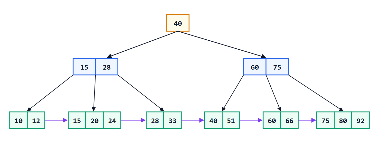
The most used index is the B+ tree: a balanced tree in which each node occupies a page and contains many sorted keys with pointers to the children. The leaves contain the keys with references to the rows (or the rows themselves) and are linked in a sorted list. Every node except the root is at least half full, and all leaves are at the same depth.
Theorem. A B+ tree with  keys in its leaves, in which each internal node has at most
 children and at least
 (the root at least 2), has a height
 satisfying

Proof. *Lower bound.* Each level multiplies the number of nodes by at most , so a tree of height has at most  leaf positions: to hold keys one needs
 , i.e.
 . *Upper bound.* The root has at least 2 children and every other internal node at least : at the leaf level there are at least
 nodes, hence (with leaves at least half full) at least as many portions of keys. From
 it follows that
 . ∎
The point is the fan-out : with 8 KB pages and 40-byte keys with pointers, is about 200. Example. With  keys,
 : 4 levels suffice, and even in the worst case, with half-full nodes, 5 are needed. The first two or three levels, a few thousand pages, always sit in the buffer: finding one row among a billion costs one or two disk reads. Insertions and deletions keep the tree balanced by splitting full nodes and merging underfull ones, at a cost that is logarithmic too.
The linked leaves also make range searches efficient (“marks between 25 and 28”, “March’s orders”) as well as sorting: find the first value and walk the list.
Hash indexes
A hash index computes from each key, with a hash function, the number of the bucket in which to look for it: on average a single access, regardless of table size. But it works only for equality searches: keys are scattered randomly among the buckets, and it is no use for ranges and sorting. That is why DBMSs almost always use B+ trees, and hash indexes in particular cases, such as in-memory joins.
Primary, secondary and composite indexes
A primary (or clustered) index determines the physical order of the rows in the table: rows with nearby keys are in the same pages, and a range is read with a few consecutive pages. There can be only one. Secondary indexes contain references to scattered rows: reading many rows through a secondary index can cost more than a scan, a different page for each row.
A composite index on several columns, for instance (surname, first_name), is sorted first by surname and, for equal surnames, by first name. It serves searches by surname, or by surname and first name, but not those by first name alone, which is scattered throughout the index: this is the leftmost prefix rule.
The price of indexes
Every index speeds up reads but slows down writes: every insertion, update or deletion must update all the table’s indexes, and every index takes space. So the columns actually used in search conditions and joins are indexed, in particular foreign keys, and not every column “just in case”.
The optimiser
For every query the DBMS evaluates many equivalent execution plans (which index to use, in what order to join the tables, with which join algorithm) and chooses the one with the lowest estimated cost, using statistics on the data: number of rows, distinct values, distribution. An index pays off when the condition is selective, i.e. it selects a small fraction of the rows, typically less than 5-10 %; otherwise a sequential scan is faster. The EXPLAIN command shows the chosen plan, and it is the first tool when a query is slow: often one discovers a full scan where an index was expected, because of an unindexed column or a condition written in a way that prevents the index from being used, such as a function applied to the column.