Queueing theory: Little's law, the M/M/1 queue and statistical multiplexing
Utilisation, Little's law with proof, the M/M/1 queue with distribution and delay proved, growth of delay with load, a numerical example, the advantage of statistical multiplexing proved.
In a packet network the largest and most variable delays arise in queues: a router receives packets from many directions and must transmit them one at a time. How long does one wait on average? How heavily can a link be loaded before delays explode? Queueing theory answers with simple and surprisingly useful formulas. In this lesson we look at Little’s law with its proof, the M/M/1 queue with the proof of the distribution of the number of packets, the growth of delay with load, and the advantage of statistical multiplexing proved.
The model
A queue is described by how customers (packets) arrive, how long service (transmission) lasts and how many servers there are. Let  be the arrival rate (packets per second) and
 the service rate (packets per second the link transmits when busy). The ratio

is the utilisation: the fraction of time the link is busy. For the queue not to grow without bound,  is needed.
Little’s law
Theorem (Little). In a system in equilibrium, the mean number of customers present  , the arrival rate and the mean time spent in the system
 are related by

Proof (idea). Observe the system for a long time  . Plot the number of customers present as a function of time and compute the area under the curve. It can be computed in two ways: integrating the number present over time,
 ; or adding up the time each customer spent in the system, because each contributes to the area a strip of height 1 and length equal to its stay. In time about
 customers arrive, with mean stay , for an area
 . Equating and dividing by gives the law. ∎
It holds for any distribution of arrivals and services, and for any part of the system: the queue alone, the server alone, a whole network. If a router holds 50 packets on average and 10 000 arrive per second, each stays 5 ms on average.
The M/M/1 queue
The simplest model has Poisson arrivals (independent, with exponential inter-arrival times), exponential service times and a single server: it is written M/M/1. The state is the number  of packets present.
Theorem. In equilibrium the probability of finding packets is  , and

Proof. The state goes from to  with an arrival, at rate , and from to with a departure, at rate . In equilibrium the probability flow between two adjacent states balances:
 , i.e.
 , whence
 . The probabilities must sum to 1:
 , so
 . The mean of a geometric distribution of this kind is
 . Finally, by Little’s law,
 . ∎
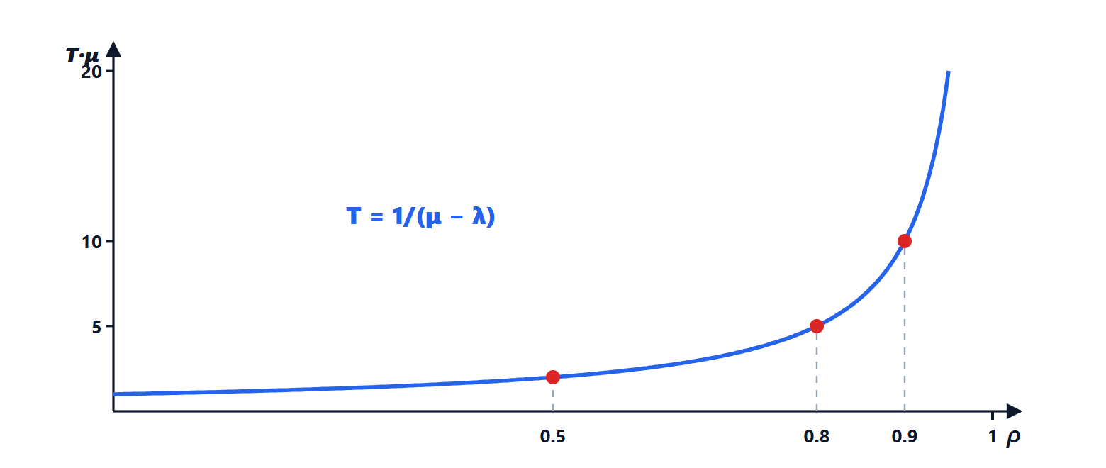
The lesson of the graph
The delay, measured in service times  , is
 : 2 at 50 % utilisation, 5 at 80 %, 10 at 90 %, 100 at 99 %. Growth is gentle up to half load and violent beyond 80 %.
Example. A 10 Mb/s link with 1000-byte packets has  packets per second, i.e. 0.8 ms per packet. With
 packets per second (
 ) the mean time in the system is
 ms: five times the transmission time. That is why network operators add capacity well before links are saturated, and why a “slow” network is often not slow but loaded.
Real traffic is not exactly Poisson: it is burstier, and delays at the same load are larger. But the shape of the curve, exploding near  , remains.
Statistical multiplexing
Theorem. A single link of capacity  shared by
 flows each of rate gives a mean delay times smaller than separate links of capacity
 , each dedicated to one flow.
Proof. With separate links, each has service rate  (where corresponds to capacity ) and arrivals :
 . With the shared link service is and arrivals
 :
 . The ratio is . Utilisation is the same in both cases. ∎
It is the quantitative justification of packet switching (lesson on architecture): pooling resources reduces waiting, because a flow can use the capacity left free by the others. The same principle, pooling resources, explains why in a supermarket a single queue serving several tills works better than separate queues.





