Doppler and coherent radars: Doppler shift, coherent and non-coherent radars, MTI and pulse-Doppler

A moving target changes the frequency of the echo: this is the Doppler effect. Measuring it gives the velocity and, above all, separates moving targets (aircraft, cars, people) from the huge echoes of stationary objects (ground, buildings, sea waves), the so-called clutter. To do so the radar must know the phase of what it transmits: this is the difference between coherent and non-coherent radars. This lesson derives the Doppler shift, explains the two architectures, and presents the two classic techniques, the MTI filter (moving target indication) and pulse-Doppler processing, with a simulation that compares them.

The idea in simple words

Everybody knows the Doppler effect from an ambulance siren: when it approaches the pitch is higher, when it moves away it is lower. Radio waves do the same, but the frequency shift is tiny, a few thousand hertz out of billions. To notice it the radar uses a trick: instead of measuring the frequency of a single pulse, it looks at how the phase of the echo changes from one pulse to the next.

The phase can be pictured as the position of a clock hand. If the target is still, each echo comes back with the hand in the same position. If the target approaches, the range gets a little shorter at every pulse and the hand moves on by a certain angle: the speed at which the hand turns is the speed of the target. To read the hand, however, the radar must know where it was when the pulse left: this is a coherent radar. A radar that starts each pulse with the hand in a random position (non-coherent) cannot do it.

The great practical advantage: stationary objects (ground, houses, mountains), which give enormous echoes, have a still hand, and can be removed by keeping only the echoes whose hand turns. This is how a car or an aircraft can be seen in front of a mountain.

The Doppler shift

Theorem. A target approaching with radial velocity shifts the echo frequency by .

Proof. The echo returns after travelling , so its phase relative to the transmitted signal is . The instantaneous frequency is the derivative of the phase divided by : , with positive if the target approaches. ∎

The 2 again comes from the round trip. The shifts are tiny compared with the carrier: a car at 30 m/s in front of a 10 GHz radar gives 2 kHz out of 10 GHz; at 77 GHz (automotive radar) 15.4 kHz; an aircraft at 250 m/s in front of a 3 GHz radar, 5 kHz. Only the radial component of the velocity counts: an aircraft crossing sideways gives no Doppler.

Coherent and non-coherent radars

A shift of a few kilohertz on a carrier of gigahertz cannot be measured within a single one-microsecond pulse: it is measured by comparing the phase of the echo from one pulse to the next. Over pulses with period , a target produces the sequence : a sinusoid “sampled” at the PRF, whose frequency is estimated with an FFT. This is possible only if the radar knows the phase each pulse started with.

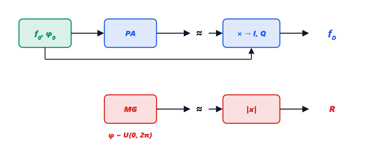
Coherent radar. The whole radar is locked to a very stable oscillator (the STALO, stable local oscillator, and the COHO, coherent oscillator, in classic radars; a single clock reference in digital radars). Every pulse leaves with a known phase, and the receiver measures the signal as a complex number, with in-phase and quadrature components (I/Q). The transmitter must be an amplifier (klystron, travelling wave tube, solid-state transistors) that amplifies a signal generated with known phase. Practically all modern radars are coherent: airborne pulse-Doppler radars, Doppler weather radars, automotive radars, SAR.

Non-coherent radar. The transmitter is a power oscillator, typically a magnetron, which starts with a random phase at every pulse. The receiver detects only the amplitude (the envelope) of the echo. It is simple and cheap, and measures range and direction well: it is the navigation radar of boats, and the surveillance radars of the first decades were like this. But it cannot measure Doppler, and cannot separate a moving target from a fixed echo in the same cell. A middle way is the coherent-on-receive radar: the phase of each transmitted pulse is sampled and subtracted from the echo, recovering coherence afterwards (with lower performance than a true coherent radar).

The MTI filter

The simplest way to remove fixed echoes is to subtract two consecutive pulses: . A stationary echo is the same from one pulse to the next and cancels; a moving echo changes phase and survives.

Theorem. The two-pulse canceller has response .

Proof. It is an FIR filter with ; on the unit circle, with , with . ∎

The response is zero at zero frequency (stationary clutter) but also at all multiples of the PRF: targets with disappear. These are the blind speeds 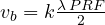: at 10 GHz with a PRF of 1 kHz, 15 m/s, 30 m/s, … The remedy is to alternate different PRFs (staggered PRF), so that a speed blind for one is not blind for the other. Three-pulse cancellers () widen the “notch” around zero, useful when the clutter is not perfectly still (trees moved by the wind, waves).

Pulse-Doppler processing

Instead of subtracting, an FFT over pulses is computed for each range cell: each FFT output is a filter centred on a velocity. Velocity resolution ; unambiguous velocity (the FFT of samples at the PRF sees frequencies from to ). With 64 pulses at 1 kHz in X band: 0.23 m/s resolution, ±7.5 m/s without ambiguity.

Choosing the PRF. Unambiguous range and unambiguous velocity go in opposite directions: their product is fixed, .

• Low PRF (a few kHz): range without ambiguity, velocity very ambiguous. Surveillance radars.
• High PRF (hundreds of kHz): velocity without ambiguity, range very ambiguous. Airborne radars against fast targets.
• Medium PRF: both ambiguous, and the ambiguities are resolved using several PRFs (with a reasoning similar to the Chinese remainder theorem). It is the choice of modern fighter radars.

The result of the processing is a range-Doppler map, the basic image of almost all coherent radars (it will appear again in the FMCW car radar).

Summary

• A target approaching with radial velocity shifts the echo frequency by ; only the velocity component along the line of sight counts.
• Doppler is measured by comparing the phase of the echo from pulse to pulse: a coherent radar is needed.
• The MTI filter subtracts consecutive pulses and cancels stationary echoes, but has blind speeds, which are avoided by changing the PRF.
• Pulse-Doppler processing (FFT over the pulses) separates targets by velocity and produces the range-Doppler map.
• Unambiguous range and velocity conflict through the PRF: low, medium or high depending on the mission.

The simulation

A range cell contains a building (fixed echo, 1000 times stronger in amplitude, that is 60 dB) and a target approaching at 5 m/s. Radar at 10 GHz, PRF 1 kHz, 64 pulses, some noise.

• Coherent with FFT: the target appears at 4.92 m/s (the true velocity, quantised to the 0.23 m/s resolution), 60 dB below the peak of the building but at a different position in the spectrum: separated.
• MTI: the fixed echo cancels completely (in this simulation it is perfectly still), the target passes with a gain of 1.73.
• Non-coherent: with a random phase at every pulse, the spectrum becomes flat: the echo of the building “smears” over all velocities and covers the target. The amplitude, the only thing the radar measures, fluctuates by only 0.07 %: the target cannot be seen.

import numpy as np

c, f0, PRF, N = 299792458.0, 10e9, 1e3, 64            # X band, PRF 1 kHz, 64 pulses
lam, T = c / f0, 1 / PRF
rng = np.random.default_rng(0)
n = np.arange(N)

v = 5.0                                                # target approaching at 5 m/s
fD = 2 * v / lam                                       # Doppler shift
target_echo = 1.0 * np.exp(1j * 2 * np.pi * fD * n * T)
fixed_echo = 1000.0 * np.exp(1j * 0.3)                 # clutter: a building, 60 dB stronger and still
noise = (rng.normal(size=N) + 1j * rng.normal(size=N)) * 0.05
x = target_echo + fixed_echo + noise                   # samples in the same range cell, pulse by pulse

def spectrum(s):
    S = np.abs(np.fft.fftshift(np.fft.fft(s * np.hanning(N))))
    return 20 * np.log10(S / S.max() + 1e-12)
vel = np.fft.fftshift(np.fft.fftfreq(N, T)) * lam / 2      # velocity axis

print(f"f_D = {fD:.0f} Hz; velocity resolution {lam / (2 * N * T):.3f} m/s; unambiguous velocity +-{lam * PRF / 4:.1f} m/s")
# 1) coherent radar: FFT over the pulses, the target separates from the fixed echo
S = spectrum(x)
k = np.argmax(np.where(np.abs(vel) > 1, S, -999))
print(f"coherent: target at {vel[k]:.2f} m/s, {S[k]:.1f} dB relative to the fixed echo peak")
# 2) two-pulse MTI: y_n = x_n - x_(n-1) cancels what does not move
y = x[1:] - x[:-1]
print(f"MTI: fixed echo power reduced from {np.mean(np.abs(fixed_echo) ** 2):.0f} to {np.mean(np.abs(np.diff(np.full(N, fixed_echo))) ** 2):.0f}; "
      f"gain on the target |H| = {2 * abs(np.sin(np.pi * fD / PRF)):.2f}")
print(f"MTI blind speed: {lam * PRF / 2:.1f} m/s")
# 3) non-coherent radar: every pulse starts with a random phase (magnetron), only the amplitude is measured
phase = np.exp(1j * rng.uniform(0, 2 * np.pi, N))
xn = x * phase
amp = np.abs(xn)
Sn = spectrum(xn)
print(f"non-coherent: amplitude fluctuation {amp.std() / amp.mean() * 100:.2f} %, no Doppler peak (maximum away from zero {Sn[np.abs(vel) > 1].max():.1f} dB, flat)")

Running it prints Hz, 0.234 m/s resolution and ±7.5 m/s unambiguous span; for the coherent radar the target at 4.92 m/s, 60.3 dB below the fixed echo; for the MTI the fixed echo cancelled and a gain of 1.73 on the target, with a blind speed of 15 m/s; for the non-coherent radar a fluctuation of 0.07 % and a flat spectrum, whose maximum (0 dB) falls far from zero velocity.