Solved exercises on radar systems: radar equation in dB, Doppler, compression, blind speeds, arrays, clutter, FMCW and SAR
Ten exercises at three levels with step-by-step solutions and graphs: range and second trace, budget in decibels, Doppler, pulse compression, staggered PRFs, fluctuating targets, array design, MTI and phase noise, an FMCW car radar, a real satellite SAR.
Exercises on radar systems of the kind found in exams, at three levels: basic, with the fundamental formulas (range, radar equation in decibels, Doppler, pulse compression); intermediate, with design choices (blind speeds, detection, arrays, clutter); exam, with the design of an automotive radar and the analysis of a real satellite SAR. Constants:  m/s,
 dBm/Hz. The result is given at once; the full solution, step by step and with the graph, opens with a click. The proofs of the formulas are in the lessons of the course.
Basic level
Exercise 1. Range and ambiguity
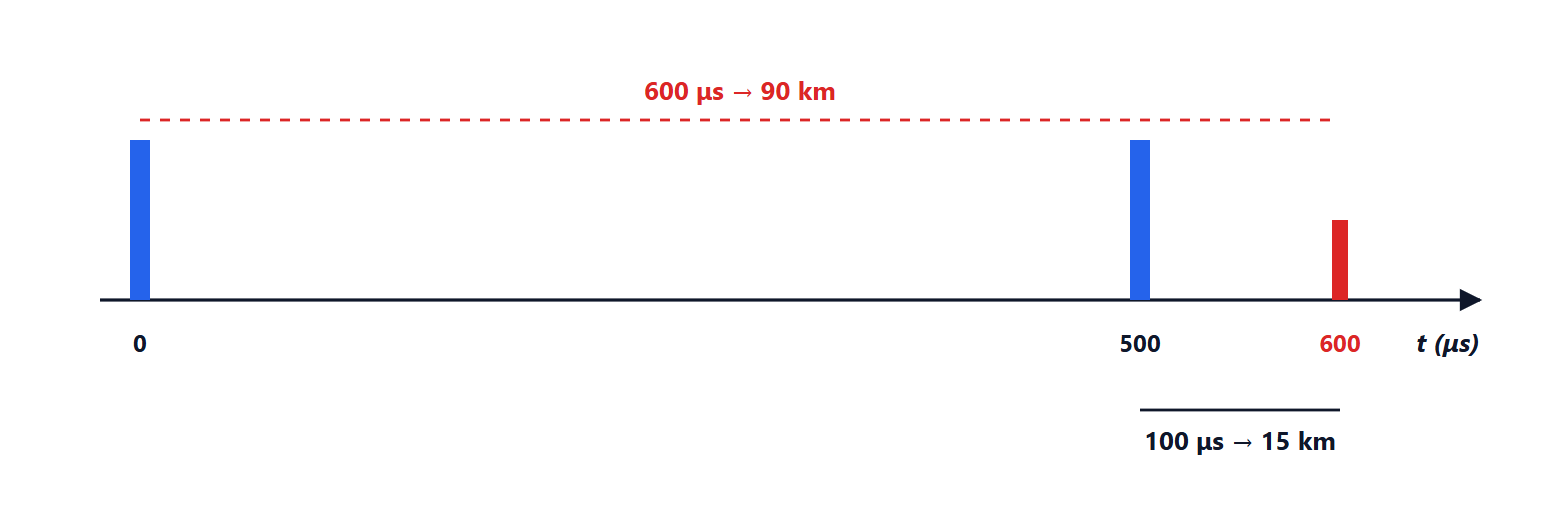
A radar receives an echo 400 μs after transmitting a pulse. How far is the target? If the radar transmits with a PRF of 2 kHz, what is the unambiguous range, and where does a target located at 90 km appear?
Result: 60 km; 75 km; the target at 90 km appears at 15 km.
Solution
1. The wave makes a round trip:  km. A handy rule to remember: 150 m per microsecond, so 400 μs give
 m.
2. Between two pulses  μs elapse. An echo arriving before the next pulse is attributed correctly; the maximum unambiguous range is
 km.
3. The target at 90 km answers after  μs, that is 100 μs after the next pulse. The radar attributes it to that pulse and places it at
 km:
 km. It is a “second-trace” target. To unmask it, the PRF is changed from one group of pulses to the next: a true target stays at the same range, the second-trace one jumps.
Exercise 2. The radar equation in decibels
An S-band radar (3 GHz) transmits 100 kW peak with a 30 dB antenna. Compute the power received from a 2 m² aircraft at 50 km, and the signal-to-noise ratio with 1 MHz of bandwidth and a 3 dB noise figure.
Result:  dBm; noise −111.0 dBm; SNR = 13.0 dB.
Solution
1. In decibels the radar equation  becomes a sum. With
 m:
| term | value | dB |
|---|---|---|
 | 100 kW | +80.0 dBm |
 | 30 dB twice | +60.0 |
 | 0.01 m² | −20.0 |
 | 2 m² | +3.0 |
 |  | −33.0 |
 |  m | −188.0 |
Sum: dBm, that is  W.
2. The noise:  dBm.
3.  dB: exactly the value needed for
 and
 with one pulse (lesson on detection). 50 km is therefore the range of this radar for this aircraft, without integration and without losses. With 6 dB of losses the range would drop by
 times, to 35 km; integrating 10 pulses (about 8 dB) would bring it back up.
Exercise 3. The Doppler of a car
A 24 GHz police radar measures a car approaching at 120 km/h. What is the Doppler shift? And if the radar is at the side of the road and sees the car at an angle of 30° to the direction of travel?
Result: 5.34 kHz; 4.62 kHz (the measured speed would be 104 km/h).
Solution
1.  cm,
 m/s:
 kHz.
2. Doppler sees only the radial component:  m/s,
 kHz. The radar, if it does not know the angle, measures
 km/h: the cosine error always favours the driver (the measured speed is less than or equal to the true one). This is why Doppler speed cameras are installed at small, known angles, and the correction is applied by design.
Exercise 4. Pulse compression
A radar transmits a 50 μs chirp with 5 MHz of bandwidth. Compute the compression ratio, the range resolution and the blind zone in front of the radar. How long would a simple pulse with the same resolution be, and how much more peak power would be needed for the same energy?
Result:  ; 30 m; 7.5 km; a 0.2 μs pulse with 250 times the peak power (+24 dB).
Solution
1.  .
2. After the matched filter the resolution depends only on bandwidth:  m.
3. While transmitting, the radar does not receive: the blind zone is  km. For close targets a short pulse is added.
4. A simple pulse with the same resolution lasts  μs; for the same energy
 a peak power
 times higher would be needed, that is 24 dB. This is exactly the advantage of compression.
Intermediate level
Exercise 5. Blind speeds and staggered PRF
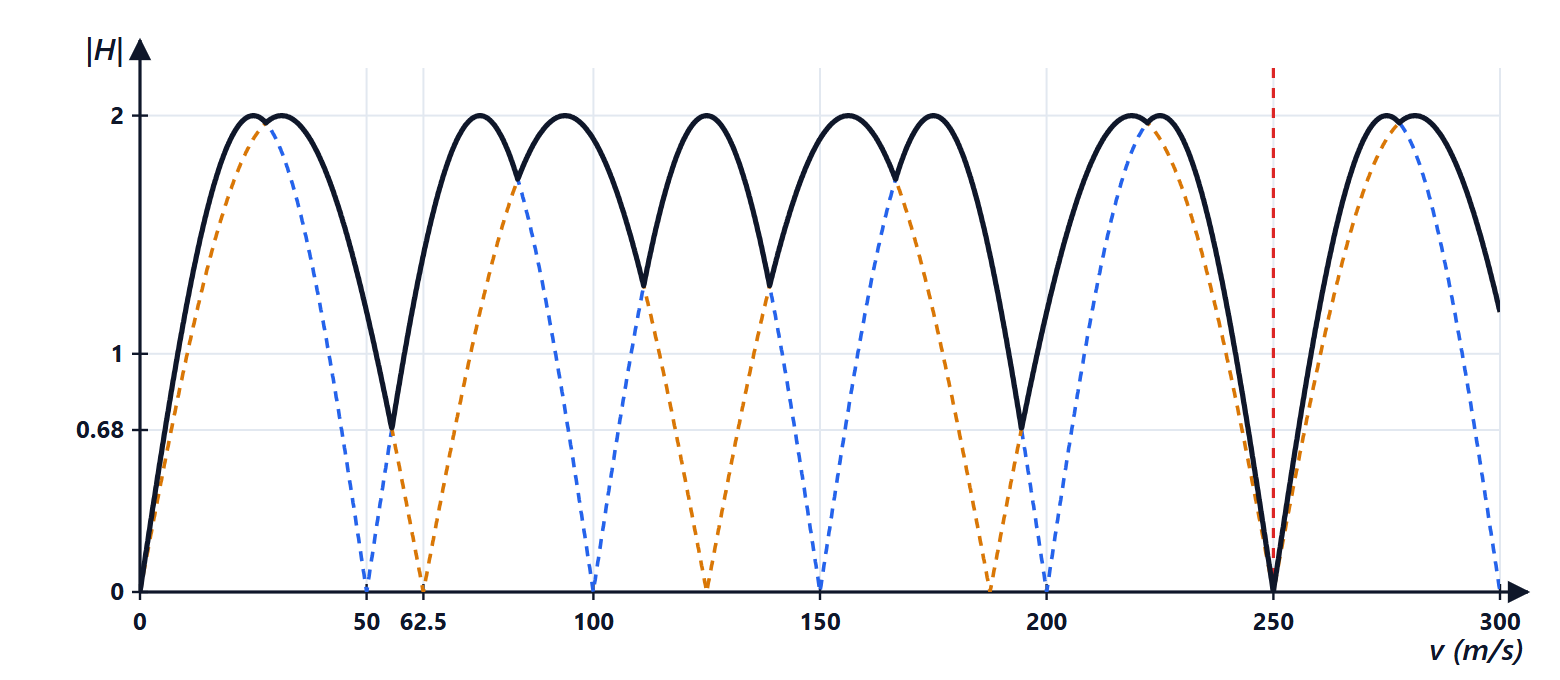
An S-band surveillance radar (3 GHz) uses a two-pulse MTI canceller. Compute the first blind speed with a PRF of 1000 Hz and of 1250 Hz. Alternating the two PRFs, what is the first common blind speed? In the range from 20 to 240 m/s, what is the worst response when the better of the two PRFs is chosen for each speed?
Result: 50 m/s and 62.5 m/s; 250 m/s; 0.68, that is −3.3 dB relative to unit gain.
Solution
1. The  canceller has response
 , zero for
 . With
 and
 m:
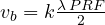 , that is 50 m/s (and multiples) with 1000 Hz, 62.5 m/s with 1250 Hz.
2. A speed is blind for both if it is a multiple of both 50 and 62.5: the least common multiple is 250 m/s. The 4:5 ratio between the PRFs multiplies the first blind speed by 5 compared with 1000 Hz. With three well-chosen PRFs one gets beyond the speeds of the targets of interest.
3. Computing the maximum of the two responses on a fine grid, the minimum value between 20 and 240 m/s is 0.68, that is −3.3 dB, at the points where the two responses cross (at 55.6 and 194.4 m/s): no speed of interest is lost, at the cost of a few decibels in some zones. Below 20 m/s the response falls towards zero anyway: it is the notch that removes stationary clutter.
Exercise 6. Constant and fluctuating target
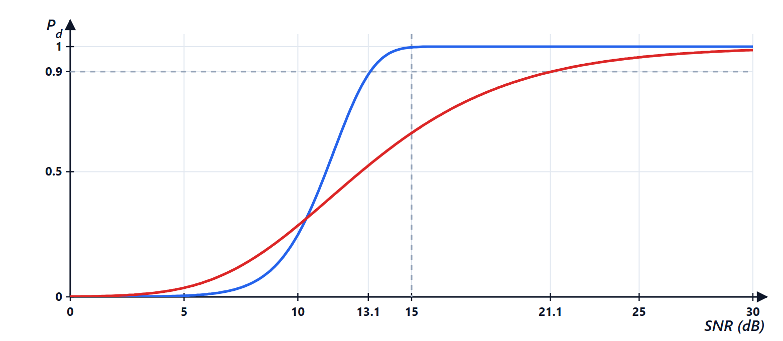
With and an SNR of 15 dB on a single pulse, compute  for a constant target and for a Swerling 1 target. With how many dB per pulse is obtained (constant target) integrating 10 pulses non-coherently?
Result: 0.997 (constant); 0.655 (Swerling 1); 5.0 dB per pulse.
Solution
1. Constant target: the threshold is  ; with SNR = 31.6 the echo amplitude is
 , well above the threshold. Marcum’s function gives
 .
2. Swerling 1:  . With the same mean SNR, the fluctuating target is lost one time in three: in the looks where its radar cross section is small, the echo stays below the threshold.
3. Albersheim with  :
 dB, with
 ,
 . Against the 13.1 dB of a single pulse, integration gains 8.1 dB.
Exercise 7. Designing an array
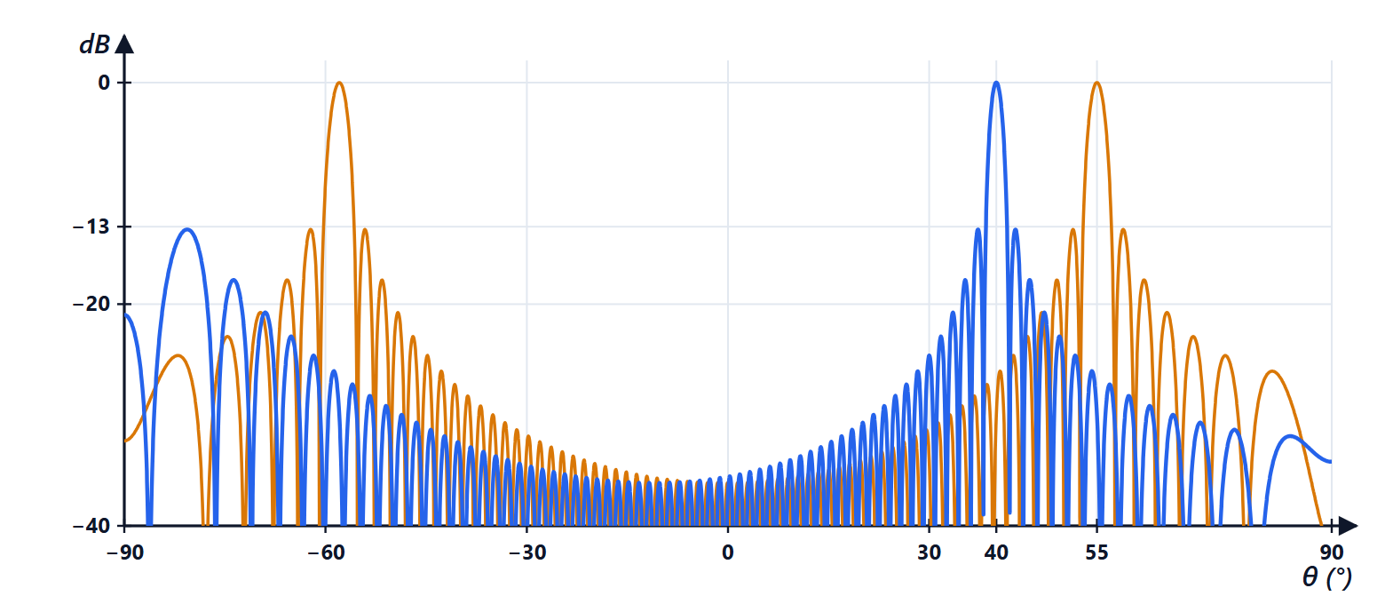
A linear array of 64 elements is spaced  . Up to what angle can it be steered without grating lobes? How wide is the beam at broadside and at 40°? What phase shift between adjacent elements is needed to steer to 40°?
Result: 41.8°; 1.32° and 1.73°; 138.8°.
Solution
1. Condition: 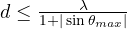 , hence
 ,
 . Spacing the elements more than half a wavelength saves (expensive) modules but limits the scan range.
2. 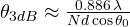 : at broadside
 rad, that is 1.32°; at 40° divide by
 : 1.73°.
3.  . With a 4-bit phase shifter (22.5° steps) 135° would be used, with a residual error that, repeating along the array, is spread with a known random phase.
Exercise 8. How much the MTI must cancel
A radar with a 1.2° beam and a 0.5 μs compressed pulse looks at a small 0.5 m² light aircraft at 30 km, over terrain with  dB. Compute the clutter radar cross section, the signal-to-clutter ratio, the improvement factor needed to reach 13 dB, and the maximum compatible transmitter phase noise.
Result:  m² (21.7 dBsm); SCR = −24.7 dB; 37.7 dB needed; phase noise below 9.2 mrad (0.53°).
Solution
1. Cell area:  m².
 m².
2.  dB: the aircraft is 300 times weaker than the clutter of its cell.
3. To reach +13 dB an improvement of  dB is needed.
4. The two-pulse canceller with phase noise  leaves a residue
 (lesson on transmitters and receivers):
 gives
 mrad. A magnetron, with random phase, would not make it even with coherent-on-receive; a coherent transmitter with a good oscillator is needed. Note that shortening the pulse (more bandwidth) shrinks the cell and directly improves the signal-to-clutter ratio.
Exam level
Exercise 9. Designing an FMCW car radar
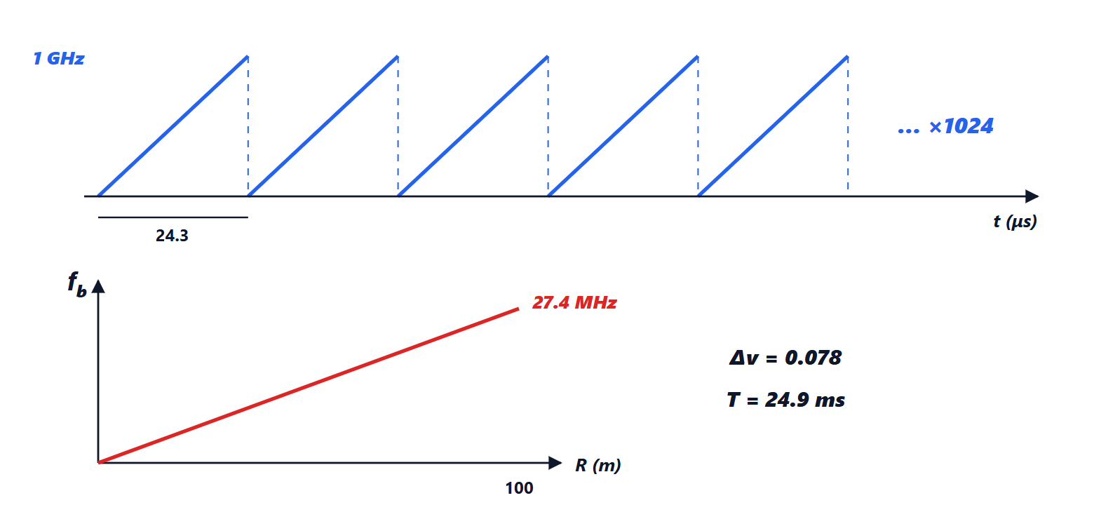
A 77 GHz radar is required with a range resolution of 15 cm, an unambiguous velocity of ±40 m/s, a velocity resolution of at least 0.1 m/s and a range of 100 m. Compute bandwidth, maximum chirp duration, number of chirps (a power of 2), frame time, chirp slope and beat frequency at 100 m.
Result:  GHz;
 μs; 800 chirps, hence 1024; 24.9 ms; 41 MHz/μs; 27.4 MHz.
Solution
1.  , hence
 GHz (within the 77-81 GHz band).
2. The unambiguous velocity is  with
 mm:
 μs.
3.  , hence
 ; with the FFT 1024 are used, giving
 m/s.
4. Frame:  μs = 24.9 ms, compatible with an update every 50 ms.
5. Slope  MHz/μs; at 100 m the beat is
 MHz: the quadrature ADC must sample at least at 27.4 MS/s (more in practice, for the anti-aliasing filter). The design shows the trade-offs: short chirps for velocity, many chirps for velocity resolution, bandwidth for range, and a fast ADC for maximum range.
Exercise 10. A real satellite SAR
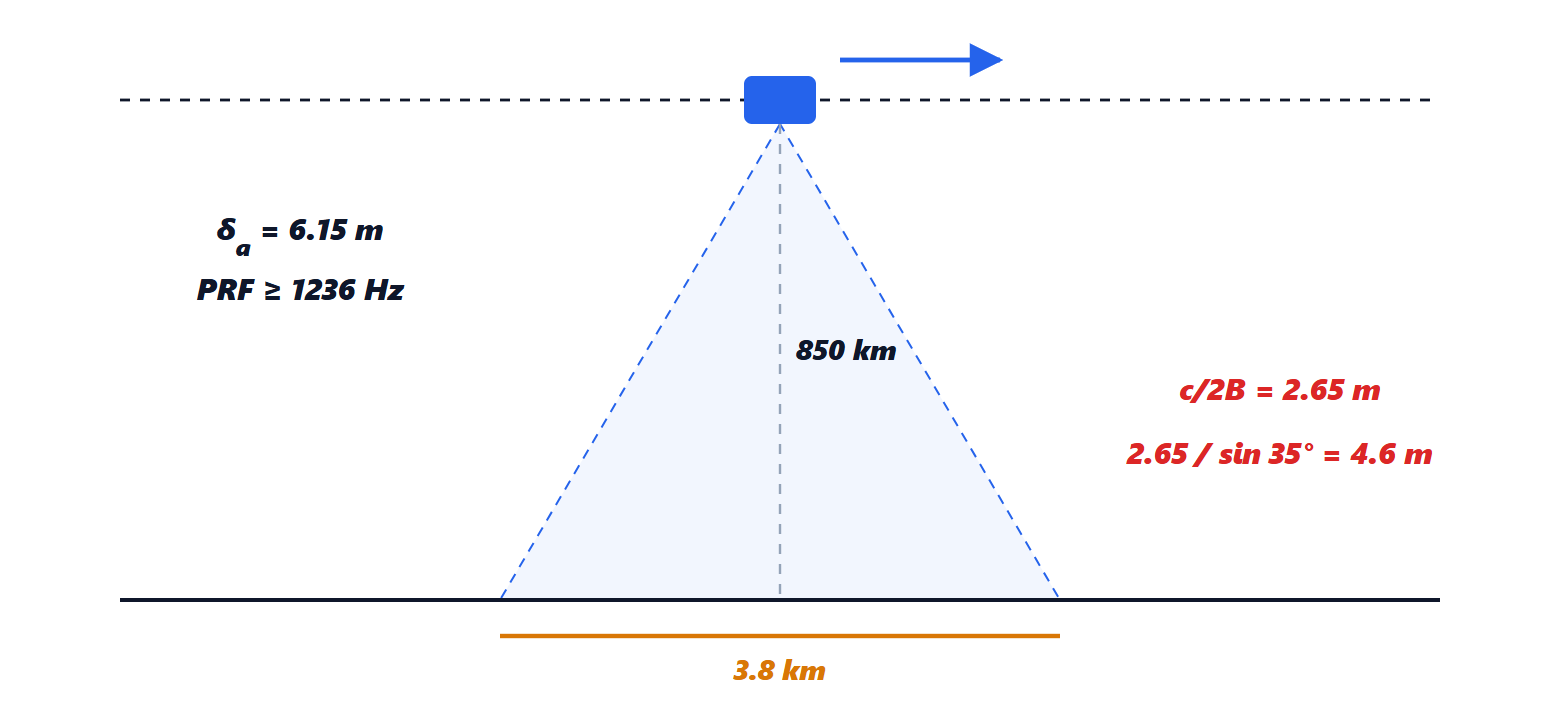
A C-band satellite (5.405 GHz) with a 12.3 m antenna flies at 7.6 km/s and observes at a range of 850 km, with 56.5 MHz of bandwidth and an incidence angle of 35° (values similar to those of Sentinel-1). Compute the azimuth resolution with the real antenna, the length of the synthetic aperture, the SAR azimuth resolution, the minimum PRF, the illumination time of a point and the slant and ground range resolutions.
Result: 3.8 km; 3.8 km; 6.15 m; 1236 Hz; 0.50 s; 2.65 m slant, 4.6 m on the ground.
Solution
1.  cm. Real antenna:
 km.
2. Each point stays in the beam for a stretch of orbit as long as the footprint:  km, travelled in
 s.
3. SAR resolution:  m, independent of range and wavelength.
4.  Hz (Sentinel-1 uses PRFs between about 1 and 3 kHz depending on the mode).
5. In slant range  m; projected on the ground, divide by
 : 4.6 m. With small incidence angles the ground resolution gets much worse (with 20° it would be 7.8 m). In wide-swath modes, to cover 250 km, the satellite divides its time among sub-swaths and the real azimuth resolution worsens to about 20 m: a trade-off between coverage and detail.