SAR, weather radars and military radars: synthetic aperture, reflectivity, jamming and burn-through
The D/2 resolution of synthetic aperture radar proved and simulated, the PRF condition and azimuth aliasing, InSAR, weather radar reflectivity and dual polarisation, the jamming equation and burn-through, countermeasures, LPI and radars against stealth.
Three families of radar show how the same principle adapts to different purposes. Synthetic aperture radar (SAR) photographs the Earth from satellites with one-metre resolution, by day and night, through clouds. Weather radars measure rain and wind inside thunderstorms. Military radars must work against an adversary trying to blind or deceive them, and this has given rise to electronic warfare. This lesson derives the SAR resolution and the sampling condition, presents meteorological reflectivity and polarimetry, and the jamming equation with the “burn-through” range, with the main countermeasures. Military aspects are treated at the level of the open, educational literature.
The idea in simple words
To see small details from far away a very large antenna is needed: to distinguish one-metre objects from 800 km in C band an antenna kilometres long would be required. SAR “builds” it with motion: the satellite records the echo while moving forward, and the computer combines the recordings as if they came from a single antenna as long as the path travelled. It is like photographing a panorama with many pictures taken while moving and then joining them, but also taking the phase of the waves into account.
Weather radars use the echo of raindrops, which for a radar is “noise” (clutter) but for a meteorologist is the useful signal. Military radars, finally, work against an adversary who can transmit in turn to blind or deceive them: the comparison between jamming and echo follows a simple law, which the lesson derives.
Synthetic aperture radar
A side-looking radar on a satellite illuminates a strip of ground. In range (perpendicular to the motion) the resolution is that of pulse compression,  . In azimuth (along the motion), with a real antenna of length
 , the resolution would be the beamwidth on the ground,
 : for a satellite at 800 km, in C band (
 cm), with a 2 m antenna, 22 km. Useless for imaging.
The SAR idea: as the satellite moves forward, each point on the ground stays in the beam for a stretch of orbit exactly  long (22 km). Recording the echoes with their phase (the radar is coherent) and combining them in the computer gives the equivalent of an antenna
 long: a synthetic aperture.
Theorem. The azimuth resolution of SAR is  , independent of range and wavelength.
Proof. An antenna of length has one-way angular resolution  ; but in a radar the path is a round trip and the phase changes twice as fast along the synthetic aperture, so the angular resolution is
 . At range
 this becomes
 . ∎
The result is paradoxical but true: a shorter antenna gives a better resolution, because its wider beam illuminates each point over a longer stretch. There is however a constraint: the radar must sample the aperture densely enough. The phase history of a point, during the pass, is a chirp (the range varies as  ), with a Doppler bandwidth of
 ; sampling at the PRF must satisfy the Nyquist theorem:
 , that is the satellite must not move more than
 between one pulse and the next. With
 km/s and
 m at least 7.5 kHz are needed; but the PRF cannot be too high, so as not to create range ambiguities over the illuminated swath: this is the central trade-off in the design of a spaceborne SAR.
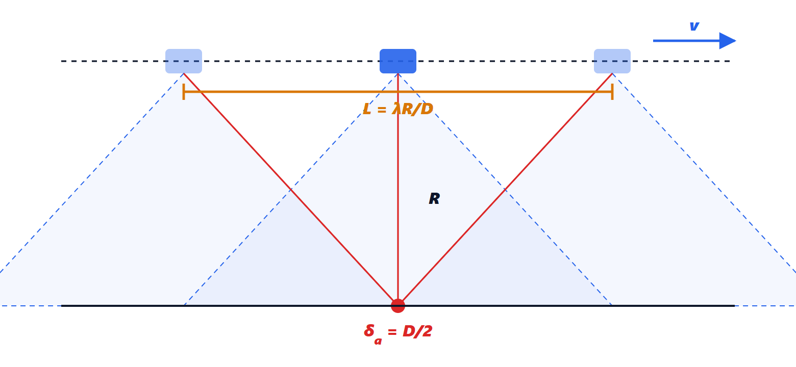
Simulation. A point on the ground, the satellite with a PRF of 15 kHz (one pulse every 0.5 m, 44 414 pulses along the aperture): combining the echoes with the expected phase (“focusing”, a matched filter along the orbit), the point has a −3 dB width of 0.88 m, against 0.89 m from theory ( ) and 22 km with the real antenna. With 5 kHz (1.5 m between pulses, more than ) the Nyquist condition is violated: a ghost copy of the point appears at
 km, still inside the illuminated area and only 6 dB below the true point (azimuth aliasing; in a real system the antenna pattern attenuates it, but not enough).
Applications. Sentinel-1 (Copernicus, C band) and COSMO-SkyMed (Italian Space Agency, X band) observe ice, seas, floods, deforestation and ships. SAR interferometry (InSAR) compares the phase of two passes: range changes of a fraction of a wavelength become measurable, and ground deformations of millimetres are measured (landslides, subsidence, volcanoes, settlement of buildings and infrastructure).
Weather radars
Raindrops, small compared with the wavelength (in S or C band), scatter according to Rayleigh’s law, with a cross section proportional to  , with
 the drop diameter. The measured quantity is the reflectivity

It depends mostly on the large drops (the sixth power). The link with the rain rate in mm/h is empirical; the most used is that of Marshall and Palmer,  : 1 mm/h gives 23 dBZ, 10 mm/h 39 dBZ, 50 mm/h 50 dBZ. Conversely 45 dBZ correspond to about 24 mm/h.
Modern weather radars are:
- Doppler: they measure the radial velocity of the drops, hence the wind inside the storm, and recognise the rotations that precede tornadoes;
- dual-polarisation: they transmit with horizontal and vertical polarisation. Large drops flatten as they fall and reflect more horizontally (positive differential reflectivity
 ); hail, irregular and tumbling, does not; snow has its own values. With , the differential phase
 and the correlation coefficient between the two polarisations, precipitation is classified and clutter is recognised (ground, birds, insects have low correlation) and removed from the maps.
Military radars and electronic warfare
Military radars perform surveillance (detection at long range), tracking and fire control, missile guidance, and ground observation from aircraft. The essential difference from civil radars is the adversary, who tries not to be seen (low radar cross section, low-altitude flight below the radar horizon, lessons on the radar cross section and on propagation) or to jam the radar.
Noise jamming. A jammer on board the target transmits noise with power  , gain
 , over a bandwidth
 . The radar receives the jamming over a one-way path (falling as
 ) and the echo over a round trip (
 ).
Theorem. For a self-screening jammer on board the target, the jamming-to-signal ratio in the radar receiver is

Proof. The received jamming is  (only the fraction
 of the noise falls within the receiver band); the signal is that of the radar equation,
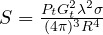 . Taking the ratio,
 , one
 and two factors
 cancel and the formula remains. ∎
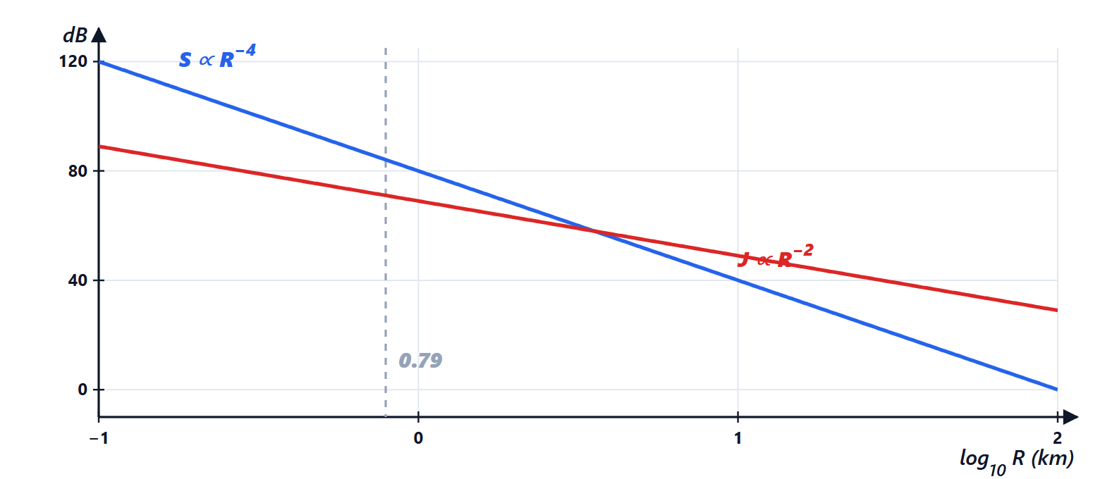
 grows as : from far away the jamming wins, getting closer the echo grows faster. The burn-through range is the one below which the radar “burns through” the jamming and detects the target. With a 100 kW, 35 dB radar, a 5 m² target and a 100 W, 10 dB jammer spreading its noise over 100 MHz (against the 1 MHz of the receiver):
 dB at 100 km, 15 dB at 20 km, 3 dB at 5 km; to have a signal 13 dB above the jamming one has to get to 0.8 km.
Countermeasures and counter-countermeasures (in general terms):
- deception: instead of noise, the jammer records the radar pulse with a digital memory (DRFM) and retransmits it modified, creating false targets or gradually moving the tracking gate (range gate pull-off). The radar defends itself with waveforms that change from pulse to pulse, with checks of the consistency between range and Doppler, with monopulse;
- frequency agility: the radar changes frequency at every pulse or group of pulses, forcing the jammer to spread its power over a wide band (increasing );
- sidelobe cancellation and adaptive nulling with the array (lesson on clutter): a null of the pattern in the direction of the jammer;
- low probability of intercept (LPI) radars: low peak power, long coded pulses and wide bandwidth, so that the radar sees targets without being easily detected by enemy receivers;
- against low observability (stealth): low-frequency radars (VHF and UHF, where shaping and absorbing materials work less well), bistatic and multistatic radars (transmitter and receiver at different places, which see the scattering in directions not designed to reduce it), and passive radars, which use existing radio and TV transmitters as illuminators and emit nothing.
Summary
- SAR synthesises an aperture long and reaches an azimuth resolution , independent of range; a PRF of at least is needed.
- SAR interferometry measures ground deformations of millimetres.
- Weather radars measure the reflectivity
 (dBZ), from which the rain rate follows; Doppler gives the wind, dual polarisation the type of precipitation.
- A self-screening jammer has
 : getting closer the echo wins (burn-through).
- Countermeasures and counter-countermeasures: DRFM deception, frequency agility, adaptive nulling, LPI, bistatic and passive radars against stealth.
The code
import numpy as np

c = 299792458.0

# 1) SAR: azimuth resolution with real and synthetic aperture
f, D, R = 5.4e9, 2.0, 800e3                          # C band, 2 m antenna, satellite at 800 km
lam = c / f
real = lam * R / D                                    # footprint of the real beam on the ground
print(f"real aperture: azimuth resolution {real / 1e3:.1f} km")
print(f"synthetic aperture {real / 1e3:.1f} km long: resolution D/2 = {D / 2:.1f} m (independent of range)")

# simulation: a point on the ground, illuminated by the satellite over the whole synthetic aperture
v, PRF = 7500.0, 15000.0                              # step v/PRF = 0.5 m: satisfies v/PRF <= D/2
print(f"step between pulses {v / PRF:.2f} m (must be at most D/2 = {D / 2:.1f} m)")
xs = np.arange(-real / 2, real / 2, v / PRF)          # satellite positions during illumination
reference = np.exp(-1j * 4 * np.pi / lam * np.sqrt(R ** 2 + xs ** 2))   # expected phase for a point at x = 0
shift = np.linspace(-3, 3, 601)                       # true position of the point along azimuth
response = np.array([abs(np.vdot(reference, np.exp(-1j * 4 * np.pi / lam * np.sqrt(R ** 2 + (xs - s) ** 2)))) for s in shift])
response /= response.max()
width = np.ptp(shift[response >= 1 / np.sqrt(2)])
print(f"simulation: {len(xs)} pulses, -3 dB width of the focused point {width:.2f} m (theory 0.886 D/2 = {0.886 * D / 2:.2f} m)")

# 2) weather radar: reflectivity and rain rate (Marshall-Palmer, Z = 200 R^1.6)
for rain in (1, 10, 50):
    Z = 200 * rain ** 1.6
    print(f"rain {rain:2d} mm/h: Z = {10 * np.log10(Z):.1f} dBZ")
dbz = 45.0
print(f"{dbz} dBZ correspond to {(10 ** (dbz / 10) / 200) ** (1 / 1.6):.1f} mm/h")

# 3) electronic warfare: jamming-to-signal ratio and burn-through range for a self-screening jammer
Pt, Gt, sigma = 100e3, 10 ** 3.5, 5.0                 # radar: 100 kW, 35 dB; 5 m^2 target
Pj, Gj, Br, Bj = 100.0, 10.0, 1e6, 100e6               # jammer: 100 W, 10 dB, noise over 100 MHz
for Rk in (100e3, 20e3, 5e3):
    js = Pj * Gj * 4 * np.pi * Rk ** 2 / (Pt * Gt * sigma) * Br / Bj
    print(f"target at {Rk / 1e3:5.0f} km: J/S = {10 * np.log10(js):5.1f} dB")
Rbt = np.sqrt(Pt * Gt * sigma * Bj / (Pj * Gj * 4 * np.pi * Br) / 10 ** 1.3)
print(f"burn-through range (S/J = 13 dB): {Rbt / 1e3:.2f} km")
Running it prints 22.2 km for the real aperture and 1.0 m for the synthetic one, the 0.5 m step, 0.88 m of simulated width, 23.0, 39.0 and 50.2 dBZ, 23.7 mm/h for 45 dBZ, J/S of 29.0, 15.0 and 3.0 dB and 0.79 km of burn-through.