The digital radar: direct RF sampling, down-conversion, digital beamforming, Capon, cognitive radar
Undersampling in the Nyquist zones, quantisation and jitter, digital down-conversion, digital beamforming and Capon's method proved separating two sources closer than the beamwidth, MIMO, cognitive radar and machine learning.
For decades a radar was largely analogue hardware: oscillators, mixers, intermediate-frequency filters, detectors, phase shifters. Today the analogue-to-digital converter has moved closer to the antenna until it almost touches it, and almost everything the previous lessons described (pulse compression, Doppler, CFAR, beamforming, tracking) is software. This lesson describes the modern digital radar: direct RF sampling, digital down-conversion, digital beamforming and high-resolution estimation, MIMO radars, cognitive radar and the use of machine learning. The code samples a 3.21 GHz signal with a 2.4 GS/s converter, brings it to baseband, and separates two sources closer than the beamwidth.
The idea in simple words
A radar used to be a cabinet of circuits, each with a fixed task: filtering, converting, detecting. Today the signal is turned into numbers as soon as it leaves the antenna, and a computer does all the rest. It is the same evolution as radios turning into smartphones: the same hardware, with different programs, does different things. For radar this means forming many beams at once, changing the waveform at every pulse, adapting to the environment and using artificial intelligence to recognise targets.
From the superheterodyne receiver to direct sampling
The classic receiver is a superheterodyne: the radio-frequency signal is amplified, converted to a fixed intermediate frequency with a local oscillator, filtered, and finally detected; in coherent radars the in-phase and quadrature components (I and Q) are extracted in analogue form. Every stage introduces errors: I/Q imbalance, thermal drifts, spurious mixer products.
The converter samples at a point ever closer to the antenna:
- intermediate-frequency sampling: a single mixer, then the converter; I and Q are obtained numerically, with no imbalance;
- direct RF sampling: with converters of a few GS/s (billions of samples per second) and an analogue input bandwidth of several GHz, the signal in L, S and even C band is sampled directly, with no mixer.
Direct sampling exploits undersampling (bandpass sampling): a signal at a frequency  higher than
 appears, after sampling, at
 with
 an integer. It is not an error if the signal occupies a single Nyquist zone (the intervals wide) and an analogue filter removes the others. With
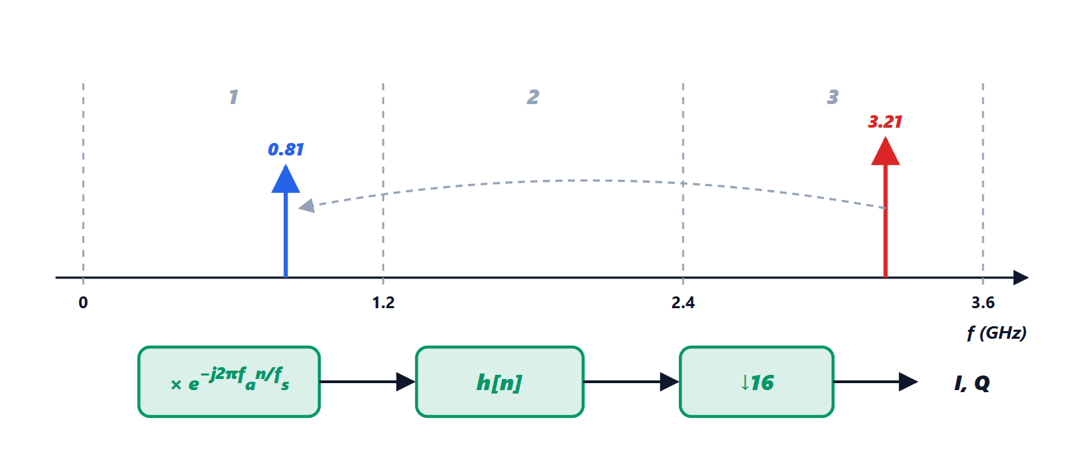
 GS/s, a 3.21 GHz signal is in the third zone (from 2.4 to 3.6 GHz) and appears at 0.81 GHz.
Quantisation. An ideal  -bit converter, with a full-scale sinusoid, has a quantisation signal-to-noise ratio

(the quantisation step  gives a uniform error of power
 , and the sinusoid of amplitude
 has power
 ; the ratio is
 ). At 12 bits it is 74 dB. Real converters have a lower effective number of bits (ENOB), because of noise and non-linearity and above all because of clock jitter: a timing error
 on a signal of frequency limits the ratio to
 , so at 3 GHz clocks with jitter of tens of femtoseconds are needed. This is why direct sampling in the higher bands is recent.
Digital down-conversion (DDC): the sampled signal is multiplied by a numerical oscillator  (NCO) that brings it to zero frequency, then filtered and decimated (one sample out of every
 is kept), because the useful bandwidth is much narrower than . The result is low-rate complex I and Q samples, on which the algorithms of the previous lessons work. In the code, decimating by 16, the rate goes from 2.4 GS/s to 150 MS/s and the phase of the signal (0.300 rad) is measured exactly.
Digital beamforming
In an analogue electronically scanned array (lesson on phased arrays) the phase shifters form one beam at a time. If instead each element (or each subarray) has its own receiver and converter, the signals of all elements reach the computer, and the beams are formed afterwards, numerically:  , with
 the vector of samples of the elements and
 the steering vector,
 .
The consequences are profound:
- many simultaneous beams from the same data: the radar listens in all directions at once, transmitting a wide beam and receiving with many narrow beams;
- adaptive nulling of jammers (lesson on clutter) and space-time clutter cancellation (STAP), which require access to the signals of the individual elements;
- high-resolution direction estimates, beyond the beamwidth limit.
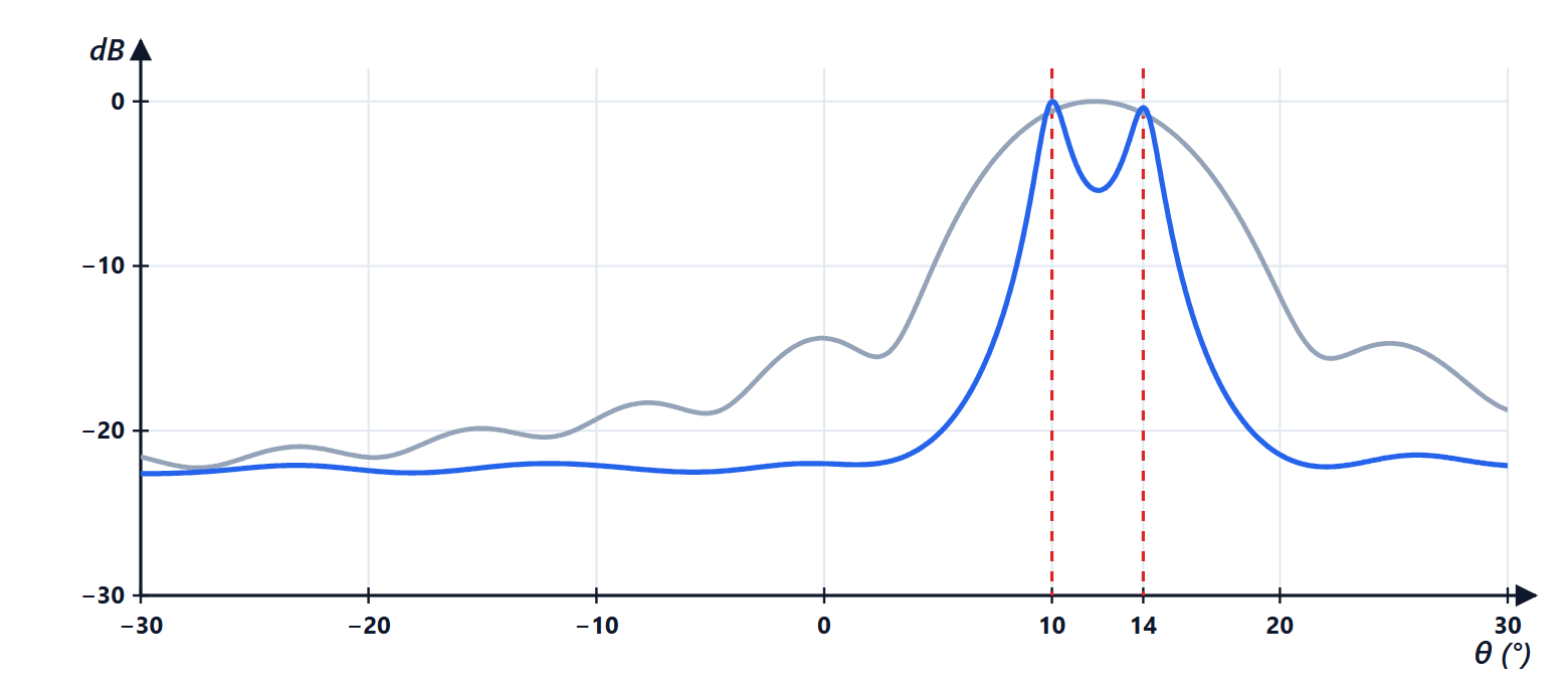
The classic beam has an angular resolution limited by the aperture: for 16 elements at  , about
 radians, that is 6.3°. Two sources at 10° and 14° fall within the same beam and are seen as a single peak. Capon’s method (MVDR, minimum variance distortionless response) computes for each direction the weights that pass direction
 without distortion and minimise the total output power:

where 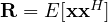 is the covariance matrix of the element signals, estimated from the data. (The solution follows from Lagrange multipliers: the gradient of
 vanishes for
 , and the constraint fixes
 .) When pointing at , Capon automatically places nulls on the nearby sources, and the two peaks separate. In the simulation (200 snapshots, 10 dB signal-to-noise ratio per element), the classic beam shows a single peak at 11.9°, while Capon finds 10.1° and 14.0° with a 5.4 dB dip between the two. Other methods of the same family, such as MUSIC and ESPRIT, exploit the eigenvector structure of
 (signal and noise subspaces). The price is the need for many snapshots and the sensitivity to array calibration errors.
MIMO radar
In MIMO radars (lesson on FMCW radars) each transmitter emits a distinguishable waveform (orthogonal in time, in frequency or by codes), and each receiver separates the contributions of the different transmitters. With transmitters and receivers a virtual array of  elements is obtained, whose positions are the sums of the transmitter and receiver positions: with 3 transmitters and 4 receivers suitably spaced, 12 virtual elements in a row. The angular resolution is that of the virtual aperture, with only 7 physical channels. The latest automotive radars (“4D radars”, also measuring elevation) reach hundreds of virtual channels with several cascaded chips.
Cognitive and software-defined radar
If everything is software, the waveform too can change from one pulse to the next. A software-defined radar uses general-purpose hardware (fast converters, FPGAs, graphics processors) and loads different functions: surveillance, tracking, mapping, even communication. The next step is cognitive radar, which closes the loop between reception and transmission:
- it chooses the waveform according to the environment: frequencies free of interference, more bandwidth where resolution is needed, longer pulses for distant targets;
- it manages resources (the radar’s time): more frequent visits to manoeuvring targets, fewer to predictable ones, search in the most likely areas;
- it shares the spectrum with communications (5G and radar use neighbouring or shared bands), also with waveforms that perform both functions together (ISAC, integrated sensing and communication, planned for 6G).
Machine learning in radar
Neural networks (Machine Learning course) enter every level of the chain:
- target classification from micro-Doppler (lesson from scan points to objects): pedestrians, cyclists, drones, birds have different Doppler-time signatures, which a convolutional network recognises as images;
- detection: networks working directly on the range-Doppler map or on point clouds, replacing or complementing CFAR and clustering;
- waveform recognition in electronic warfare receivers;
- resource management with reinforcement learning (Reinforcement Learning course): the agent decides where and how to point the radar and is rewarded by the tracking quality;
- fusion with cameras and lidar in autonomous vehicles.
The limits are the known ones: a lot of labelled data is needed (often generated with simulators), networks can fail unpredictably outside their training conditions, and in safety applications (automotive, aviation) reliability must be demonstrated. This is why classic algorithms, with their guarantees (constant false alarm rate, Kalman filters), remain the backbone, and machine learning is added where models are too complicated to write by hand.
Summary
- The converter has moved closer to the antenna: direct RF sampling with undersampling in the Nyquist zones, then digital down-conversion (NCO, filter, decimation).
- The converter dynamic range (6.02N + 1.76 dB) and clock jitter limit performance.
- Digital beamforming gives many beams at once, adaptive nulling and high-resolution estimates (Capon, MUSIC) beyond the beamwidth.
- MIMO, software-defined and cognitive radars adapt waveform and resources to the environment.
- Machine learning helps in classification, detection and resource management, alongside the classic algorithms.
The code
import numpy as np

rng = np.random.default_rng(0)

# 1) direct RF sampling: a 3.21 GHz signal sampled at 2.4 GS/s (third Nyquist zone)
fs, f0 = 2.4e9, 3.21e9
zone = int(f0 // (fs / 2)) + 1
alias = abs(f0 - round(f0 / fs) * fs)
print(f"signal at {f0 / 1e9:.2f} GHz, fs = {fs / 1e9:.1f} GS/s: Nyquist zone {zone}, appears at {alias / 1e9:.2f} GHz")
n = np.arange(8192)
bits = 12
x = 0.9 * np.cos(2 * np.pi * f0 * n / fs + 0.3) + rng.normal(0, 1e-4, len(n))
xq = np.round(x * 2 ** (bits - 1)) / 2 ** (bits - 1)                 # 12-bit converter
spectrum = np.abs(np.fft.rfft(xq * np.hanning(len(n))))
peak = np.argmax(spectrum) * fs / len(n)
err = xq - x
snr = 10 * np.log10(np.mean((0.9 * np.cos(2 * np.pi * f0 * n / fs + 0.3)) ** 2) / np.mean(err ** 2))
print(f"FFT peak at {peak / 1e9:.3f} GHz; quantisation SNR {snr:.1f} dB (theory 6.02 N + 1.76 + 20 log 0.9 = {6.02 * bits + 1.76 + 20 * np.log10(0.9):.1f} dB)")

# digital down-conversion: numerical oscillator (NCO), filter and decimation by 16
nco = np.exp(-2j * np.pi * alias * n / fs)
bb = xq * nco
h = np.hamming(129); h /= h.sum()                                    # FIR low-pass filter
bb = np.convolve(bb, h, "same")[::16]
print(f"after decimation by 16: {len(bb)} complex samples at {fs / 16 / 1e6:.0f} MS/s, measured phase {np.angle(np.mean(bb[10:-10])):.3f} rad (true 0.300)")

# 2) digital beamforming: 16 elements at half a wavelength, two sources at 10 and 14 degrees
N, d = 16, 0.5
ang = np.radians([10.0, 14.0])
steer = lambda th: np.exp(2j * np.pi * d * np.arange(N)[:, None] * np.sin(np.atleast_1d(th)))
K = 200                                                              # snapshots
S = (rng.normal(size=(2, K)) + 1j * rng.normal(size=(2, K))) / np.sqrt(2)
noise = (rng.normal(size=(N, K)) + 1j * rng.normal(size=(N, K))) / np.sqrt(2) * 10 ** (-10 / 20)
X = steer(ang) @ S + noise                                           # SNR 10 dB per element
Rxx = X @ X.conj().T / K
grid = np.radians(np.linspace(-30, 30, 1201))
A = steer(grid)
beam = np.real(np.sum(A.conj() * (Rxx @ A), axis=0)) / N ** 2        # all the beams at once, from the same data
Ri = np.linalg.inv(Rxx)
capon = 1 / np.real(np.sum(A.conj() * (Ri @ A), axis=0))             # Capon (MVDR)
def peaks(p):                                                        # local maxima within 3 dB of the highest
    i = np.where((p[1:-1] > p[:-2]) & (p[1:-1] > p[2:]))[0] + 1
    return np.degrees(grid[i[p[i] > p.max() / 2]])
print(f"-3 dB beamwidth: {np.degrees(0.886 * 2 / N):.1f} degrees, sources 4 degrees apart")
for name, p in (("classic beam", beam), ("Capon", capon)):
    between = p[(grid > np.radians(10.5)) & (grid < np.radians(13.5))].min()
    print(f"{name:15s}: peaks at {np.round(peaks(p), 1)} degrees, minimum between the sources {10 * np.log10(between / p.max()):.1f} dB")
Running it prints the third Nyquist zone and the signal at 0.81 GHz, a 73.0 dB quantisation signal-to-noise ratio (theory 73.1 dB for an amplitude of 0.9 of full scale), 512 complex samples at 150 MS/s with the phase of 0.300 rad, a 6.3° beam, a single peak at 11.9° for the classic beam and the two peaks at 10.1° and 14.0° for Capon.