Detection: threshold and false alarm, probability of detection, pulse integration and CFAR proved

A weak echo buried in noise must be detected: the radar has to decide, cell by cell, whether a target is there or not. Every decision can go wrong in two ways: missing a target that is there (missed detection) or reporting one that is not (false alarm). This lesson sets detection up as a statistics problem, derives the threshold for a desired false alarm probability, computes the probability of detection and the required signal-to-noise ratio, explains the integration of several pulses, and proves how CFAR works, the detector that adapts the threshold to the actual noise, found in every modern radar.

The idea in simple words

Imagine listening to a radio with a lot of hiss and having to say whether someone spoke at a certain instant. If you say “yes” every time the hiss rises a little, you will often be wrong, claiming a voice that was not there (false alarm). If you say “yes” only when the sound is very loud, you will miss the faint voices (missed detection). A threshold has to be chosen, and the choice is always a compromise.

The radar makes this choice millions of times per second, once per “cell” (each combination of range, direction and velocity). Since there are so many cells, false alarms must be extremely rare, one in a million or fewer, otherwise the screen would fill with ghost targets. The lesson answers three questions: where to put the threshold, how strong the echo must be to be seen almost always, and how to adjust the threshold automatically when the noise changes (CFAR).

Two words about “cell” and “power”, which we will use often: for each cell the radar computes a number, the amplitude of the echo after the matched filter; its square is the power. With noise only this number is random; with a target it is larger on average.

Hypothesis testing

In each cell two hypotheses are compared: , noise only; , target plus noise. A quantity is computed (typically the amplitude of the matched filter output) and compared with a threshold . Performance is described by two probabilities: and . The Neyman-Pearson lemma states that, for a fixed , the test that maximises compares the likelihood ratio with a threshold; for signals in Gaussian noise this is equivalent to comparing the amplitude of the matched filter output with a threshold. In a radar is set very small (from to ): with millions of cells examined per second, even gives a few false alarms per second.

The threshold in noise

Complex noise, with independent Gaussian I and Q components of variance , has an amplitude with Rayleigh distribution.

Theorem. With noise only, ; hence the threshold for a desired is .

Proof. The joint density of I and Q is . Moving to polar coordinates (, area element ) and integrating over the angle gives the Rayleigh density . Then . ∎

For the threshold is ; for , . The dependence on the threshold is exponential: a 1 dB error in the noise estimate changes by an order of magnitude. This is the reason for CFAR.

The probability of detection

With a constant target of amplitude the amplitude follows the Rice distribution, and is expressed through Marcum’s Q function. For design, Albersheim’s empirical formula is used, giving the signal-to-noise ratio needed for the desired and when pulses are integrated non-coherently:

For and with a single pulse it takes 13.1 dB: the value used in the example of the lesson on the radar equation. A simulation with two million noise samples and the exact threshold gives of about and, with a target at 13.2 dB, , equal to Marcum’s function (0.902).

Integrating several pulses

The target stays in the beam for many pulses. Adding them improves the signal-to-noise ratio:

• coherent integration (sum of the complex values, that is the Doppler FFT of the lesson on Doppler): the signal adds in amplitude, the noise in power, the gain is exactly ;
• non-coherent integration (sum of amplitudes or powers, after the detector): simpler and independent of phase, but less efficient. With Albersheim, for and the SNR per pulse needed drops from 13.1 dB with one pulse to 5.0 dB with 10 pulses (8.1 dB gain against 10 dB for coherent integration) and to −1.3 dB with 100 (14.4 dB against 20).

Real targets fluctuate (the radar cross section changes from one look to the next): the Swerling models describe their statistics, and the same with a fluctuating target usually requires several more decibels (8 dB with one pulse for : lesson on the radar cross section).

An example to fix ideas. A surveillance radar receives 25 pulses from an aircraft while the beam sweeps past. One pulse would need 13.1 dB; integrating the 25 pulses non-coherently, 2.3 dB per pulse are enough (from Albersheim’s formula), that is 10.8 dB less: in the radar equation, with range going as the fourth root of power, the range grows by times. Integrating costs only time and computation, and it is the cheapest way to “see farther”.

CFAR

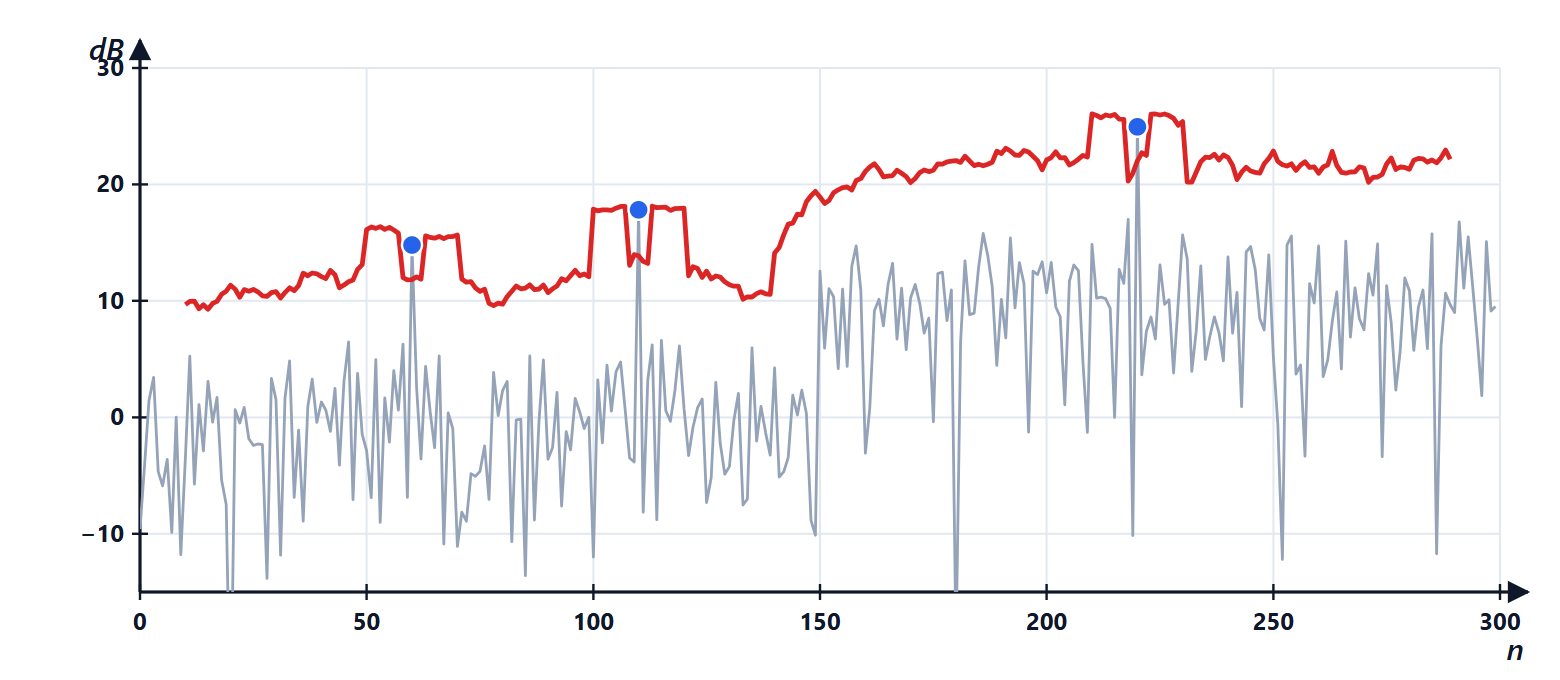
The threshold requires knowing , but the level of noise and clutter changes with range, direction, weather, interference. CFAR (constant false alarm rate) estimates the level from the cells around the one under test and sets the threshold in proportion.

CA-CFAR (cell averaging): the power is averaged over reference cells around the cell under test (excluding a few guard cells, where the echo of the target itself might be), and a target is declared if the power of the cell exceeds times the average.

Theorem. In Gaussian noise (power with exponential distribution) the CA-CFAR with cells has , independent of the noise level; hence .

Proof. Let be the sum of the reference powers and the threshold. For fixed , the probability that the cell under test (exponential with mean ) exceeds the threshold is . The sum of independent exponentials with mean has a gamma distribution, and the mean of is its generating function: . With we get : has cancelled. ∎

With and , (10.95 dB); a simulation with 400 000 trials gives . The price of the uncertainty in the estimate is the CFAR loss: if the noise were known a threshold of times the mean would suffice, so the loss is dB, which decreases as grows. The CA-CFAR suffers when another target or a clutter edge lies in the reference cells: the robust variants (OS-CFAR, GO-CFAR) are covered in the lesson on clutter filtering.

Summary

• Detection is a statistical test: the false alarm probability is fixed and the probability of detection maximised (Neyman-Pearson).
• In noise the amplitude has a Rayleigh distribution: the threshold is 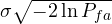, 5.26 σ for .
• For and a single pulse needs a 13.1 dB signal-to-noise ratio (Albersheim).
• Integrating pulses reduces the ratio needed per pulse: by times coherently, a little less non-coherently.
• CFAR estimates the noise from the neighbouring cells and keeps constant, with a small loss (1.3 dB with 16 cells).

The code

import numpy as np
from scipy import stats

rng = np.random.default_rng(0)
dB = lambda x: 10 ** (x / 10)

# threshold for Pfa = 1e-6 and Monte Carlo check
pfa = 1e-6
threshold = np.sqrt(-2 * np.log(pfa))                # in units of sigma
M = 2_000_000
noise = rng.normal(size=M) + 1j * rng.normal(size=M) # I and Q with sigma = 1
print(f"threshold {threshold:.3f} sigma, simulated Pfa {np.mean(np.abs(noise) > threshold):.1e}")

# probability of detection for a constant target at 13.2 dB
A = np.sqrt(2 * dB(13.2))                            # SNR = A^2 / (2 sigma^2)
print(f"simulated Pd {np.mean(np.abs(A + noise[:200000]) > threshold):.3f}, "
      f"Marcum {1 - stats.ncx2.cdf(threshold ** 2, 2, A ** 2):.3f}")

def albersheim(pd, pfa, n=1):
    a, b = np.log(0.62 / pfa), np.log(pd / (1 - pd))
    return -5 * np.log10(n) + (6.2 + 4.54 / np.sqrt(n + 0.44)) * np.log10(a + 0.12 * a * b + 1.7 * b)
for n in (1, 10, 100):
    print(f"Albersheim, {n:3d} pulses: SNR per pulse {albersheim(0.9, 1e-6, n):.2f} dB")

# CA-CFAR: threshold factor and check
N, pfa = 16, 1e-4
alpha = N * (pfa ** (-1 / N) - 1)
p = rng.exponential(1.0, (400000, N + 1))           # powers: cell under test + N reference cells
pfa_sim = np.mean(p[:, 0] > alpha / N * p[:, 1:].sum(1))
print(f"CA-CFAR: alpha = {alpha:.2f}, simulated Pfa {pfa_sim:.1e}, loss {10 * np.log10(alpha / -np.log(pfa)):.2f} dB")

Running it prints the threshold 5.257 σ with a simulated close to (with two million trials only a few exceedances are counted, so the estimate varies), simulated and computed, Albersheim’s SNRs of 13.11, 4.99 and −1.26 dB, and for CFAR , about and 1.31 dB of loss.