Small-signal amplifiers: π and T models, common emitter, base and collector, Miller effect
Transconductance and distortion proved, equivalent π and T models, gain and resistances of the BJT and FET configurations, a two-stage amplifier computed by hand, capacitors and lower cut-off frequency, Miller effect and upper cut-off frequency, checked with SPICE.
Once biased, the transistor amplifies small variations around its operating point. For small enough variations its exponential or square-law relations can be replaced by straight lines, and the transistor becomes a linear circuit made of resistors and controlled sources: the small-signal model. This lesson derives the π and T models of the BJT and the model of the FET, computes the gain, input resistance and output resistance of the three basic configurations (common emitter, common base and common collector, and the corresponding common source, common gate and common drain), studies the effect of the capacitors at low frequencies and of the transistor capacitances at high frequencies (the Miller effect), and puts everything together in a two-stage amplifier, computed by hand and checked with SPICE.
The idea in simple words
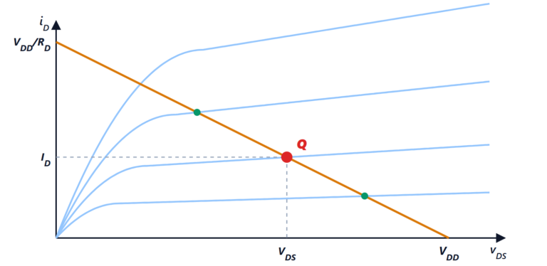
A transistor’s characteristic is curved, but every curve, looked at closely enough, looks like a straight line. If the signal is small, the transistor always works on a small piece of its curve around the operating point, and on that piece it behaves as a linear device: each extra millivolt at the input always gives the same increase in output current. The ratio between the two is the transconductance  , and almost everything depends on it. The problem is then split in two: first the DC part (biasing, previous lesson), which sets the operating point and therefore ; then the signal, on a circuit in which the transistor is replaced by its linear model.
From the curve to the line: transconductance
In a BJT in the active region  , with
 mV at room temperature.
Theorem. For small variations around the operating point  , the collector current changes by
 with

and the second-harmonic distortion, with a sinusoidal signal of amplitude  , is
 .
Proof. Let  ; then
 . The linear term is
 . With
 the quadratic term is
 : the amplitude of the second harmonic, divided by that of the fundamental
 , is . ∎
At 2 mA the transconductance is 77 mS: one extra millivolt on the base lets 77 µA more flow in the collector. “Small signal” has a precise meaning: for 1 % distortion the amplitude across the junction must stay below about 1 mV; with 10 mV the distortion is already 10 %. We will see that an unbypassed emitter resistor reduces the part of the signal that actually reaches the junction, and therefore the distortion.
In a MOSFET in saturation  , and differentiating:

At the same current the MOSFET has a much lower transconductance than the BJT: with 2 mA and  V,
 mS against 77 mS. The second-harmonic distortion, by the same reasoning, is
 : the MOSFET accepts larger signals.
The π and T models
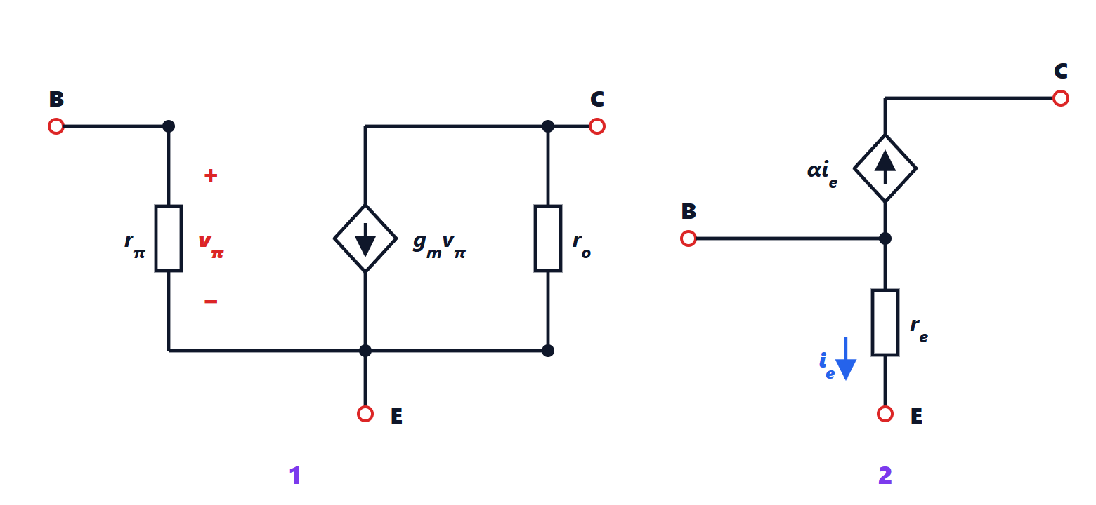
The π model (figure, 1) places between base and emitter the resistance seen from the base,  (because
 ), and between collector and emitter the source
 . The Early effect adds
 in parallel, usually tens of kΩ.
The T model (figure, 2) looks at the transistor from the emitter: the emitter current is  with
 (about 13 Ω at 2 mA), and the collector collects
 .
Theorem. The two models are equivalent.
Proof. In the T model, with  applied,
 ; the collector current is
 , equal to that of the π model. The base current is
 , because
 : the resistance seen from the base is
 , equal again. ∎
The more convenient model is used: the π model when the emitter is grounded, the T model when there is a resistor in the emitter or the signal enters at the emitter. A rule that comes from the T model and is used all the time: a resistance in the emitter, seen from the base, appears multiplied by  , and a resistance in the base, seen from the emitter, appears divided by .
The FET has the same π model without  (the gate draws no current, the input resistance is infinite) and with
 .
The method
- DC analysis: find the operating point (capacitors are open circuits).
- Parameters: , ,
 from the operating point.
- Signal circuit: DC supplies become grounds (a constant voltage source has no variation), coupling and bypass capacitors become short circuits (at the operating frequencies their impedance is negligible), transistors are replaced by their model.
- Calculation of gain and resistances with Kirchhoff’s laws.
The three BJT configurations
 denotes the total resistance seen from the collector (or the emitter) towards the load, and is neglected, since it is usually much larger than the external resistances.
Common emitter. The signal enters the base and leaves from the collector; a resistor  may remain unbypassed in the emitter (degeneration).
Theorem. In a common-emitter stage with emitter resistor

Proof. With the π model: the base current  flows through and, together with the collector current
 , through as well. Hence
 , which gives
 . The output voltage is
 ; dividing gives
 . The approximation comes from
 . Seen from the collector, the current source has infinite resistance, and
 remains. ∎
Without (bypassed emitter) the gain is  , large but dependent on current and temperature; with
 it becomes
 , a ratio of resistors: less gain, but stable, more linear (only the fraction
 of the signal reaches the junction) and with a much higher input resistance. It is negative feedback once again.
Common base. The signal enters the emitter, the base is grounded for the signal. From the T model:  (a few ohms),
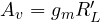 (non-inverting), current gain
 , very high
 . It is a current follower: it takes a current from a low-impedance source and delivers it unchanged into a high impedance. It is used in wideband amplifiers and in the cascode, because it does not suffer from the Miller effect.
Common collector (emitter follower). The signal enters the base and leaves from the emitter; the collector is at the supply.
Theorem. In an emitter follower with total resistance on the emitter and source resistance  seen from the base

Proof. The base current flows through and the emitter current  through :
 and
 , which give and
 . For the output resistance the signal is set to zero and a voltage
 is applied to the emitter: the resulting base current is
 , the emitter current
 times as much, and the ratio is . ∎
The gain is almost 1, but the input resistance is times the load and the output resistance times smaller than the source: it is an impedance converter (buffer), which lets a stage with high output resistance drive a low load.
The FET configurations
The same formulas hold for the FET with  (that is,
 ) and
 :
| configuration | voltage gain | input resistance | output resistance |
|---|---|---|---|
| common emitter |  |  | |
| common source |  | infinite (the gate resistors) |  |
| common base |  |  | high () |
| common gate | |  | high () |
| common collector |  |  |  |
| common drain |  | infinite | |
The FET follower (common drain) has a practically infinite input resistance but a gain noticeably less than 1 and an output resistance , that is, 100 Ω with 10 mS: much higher than that of the bipolar follower.
A complete example: two stages
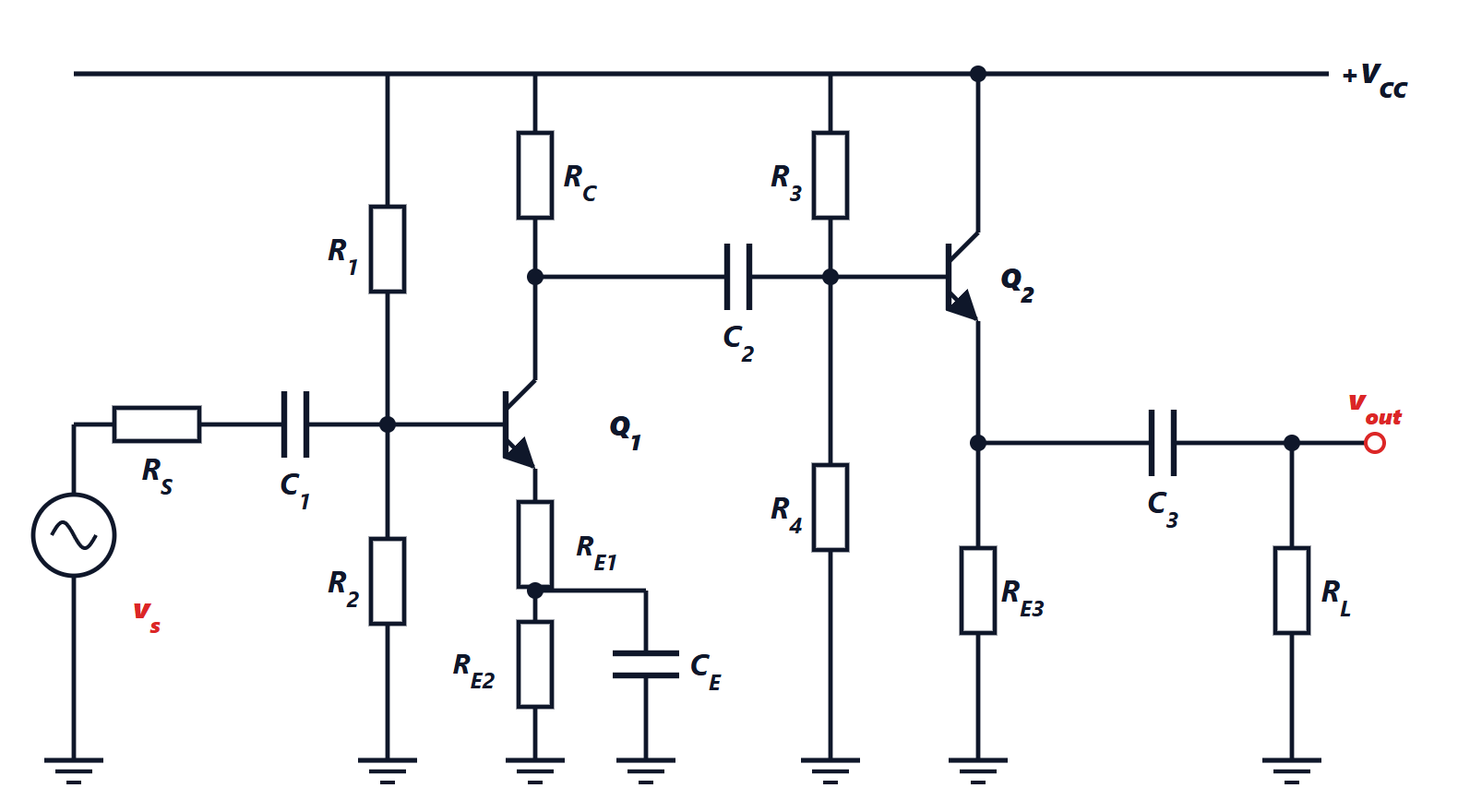
Data:  V,
 ,
 V; first stage with the divider of the biasing lesson (
 kΩ,
 kΩ,
 kΩ,
 Ω,
 kΩ); second stage with
 kΩ,
 kΩ,
 kΩ; load
 kΩ, source with
 kΩ.
DC.  mA (
 V),
 mA (
 V).
Parameters.  mS,
 kΩ;
 mS,
 kΩ;
 kΩ (negligible).
Second stage. On the emitter  Ω;
 kΩ,
 .
First stage. The collector sees  kΩ;
 kΩ,
 .
Overall. The source sees the divider  , so

and the output resistance is  Ω.
What the follower is for. Without the second stage the 1 kΩ load would sit directly on the collector:  Ω,
 and the overall gain would drop to
 . The follower gains nothing in voltage, but it almost triples the gain of the whole amplifier because it takes the load off the first stage.
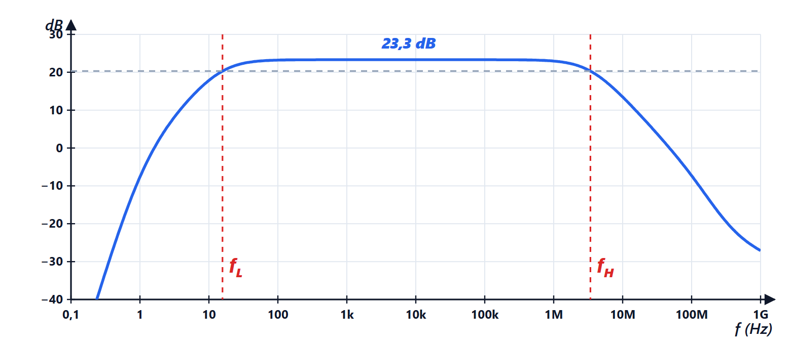
SPICE, with the complete model, gives 14.65 at mid-band (against 14.69) and an input resistance of 8.27 kΩ (against 8.26).
Low frequencies: the capacitors
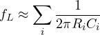
The coupling capacitors (C1, C2, C3) and the bypass capacitor (C_E) are short circuits only at high enough frequencies. Each forms a high-pass filter with the resistances it sees. The short-circuit time constant method estimates the lower cut-off frequency as follows: for each capacitor, compute the resistance it sees across its terminals with all the other capacitors shorted, and add up the poles:
| capacitor | resistance seen | pole |
|---|---|---|
| C1 = 10 µF |  = 9.26 kΩ | 1.72 Hz |
| C2 = 10 µF |  = 15.7 kΩ | 1.01 Hz |
| C3 = 100 µF |  = 1.02 kΩ | 1.56 Hz |
| C_E = 100 µF |  = 106 Ω | 15.0 Hz |
The sum gives 19.3 Hz; SPICE finds 15.8 Hz. The method overestimates a little because it adds the poles as if they were all dominant, and it neglects the zero that  creates together with
 ; but it immediately points to the critical capacitor: the emitter bypass, because it sees the very small resistance of the emitter (about
 plus the base resistances divided by ). To lower
 it is that should be increased, not the others.
High frequencies: the transistor capacitances and the Miller effect
A transistor has two capacitances:  between base and emitter (the junction capacitance plus the charge stored in the base, proportional to the current) and
 between base and collector (the reverse-biased junction, small). In the example, at the operating point, SPICE computes
 pF and
 pF. The transition frequency, at which the current gain falls to 1, is
 MHz.
Theorem (Miller). An impedance  connected between the input and the output of an amplifier with gain
 is equivalent, seen from the input, to an impedance
 to ground. For a capacitor
 with negative , the capacitance seen from the input is
 .
Proof. The current in is  , the same that an impedance between the input and ground would draw. For a capacitor
 and
 . ∎
In the first stage the gain from base to collector is about  (with
 reduced by degeneration), and the small appears multiplied by 17.8: 37 pF in parallel with the input, almost as much as . This is why high-gain common-emitter stages are slow, and why the cascode (a common base on top of a common emitter) is so widespread: it keeps the gain at the collector of the first transistor low.
The open-circuit time constant method estimates the upper cut-off frequency by adding, for each capacitance, its product with the resistance it sees with the other capacitances disconnected:
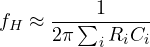
In the example:  sees 108 Ω (4.8 ns),
 sees 17.8 kΩ, the Miller effect (37.3 ns),
 4.0 ns and
 1.9 ns. The total, 48 ns, gives
 MHz; SPICE finds 3.41 MHz. The dominant term is precisely of the first stage.
Summary
- For small signals the transistor is linear:
 for the BJT,
 for the FET; “small” means a few millivolts across the BJT junction.
- The π model (
 , , ) and the T model (, ) are equivalent; a resistance in the emitter seen from the base is multiplied by .
- Common emitter: high, inverting gain,
 ; common base: low-impedance input, no Miller effect; common collector: unity gain, impedance converter.
- The band goes from , set mainly by the emitter bypass, to
 , set mainly by multiplied by the Miller effect.
- In the example: gain 14.7 (23.3 dB), band from 16 Hz to 3.4 MHz, checked with SPICE.
The code
import math

VT, beta, VA, VBE, VCC = 0.02585, 200, 100.0, 0.7, 12.0
par = lambda *r: 1 / sum(1 / x for x in r)

# first stage: common emitter with 47k/18k divider, RC 2.2k, RE1 100 ohm unbypassed and RE2 1.1k bypassed
R1, R2, RC, RE1, RE2 = 47e3, 18e3, 2.2e3, 100.0, 1.1e3
# second stage: common collector with 27k/33k divider, RE3 2.7k, load RL 1k; source with RS 1k
R3, R4, RE3, RL, RS = 27e3, 33e3, 2.7e3, 1e3, 1e3

# DC analysis
VTH1, RTH1 = VCC * R2 / (R1 + R2), par(R1, R2)
IC1 = beta / (beta + 1) * (VTH1 - VBE) / (RE1 + RE2 + RTH1 / (beta + 1))
VTH2, RTH2 = VCC * R4 / (R3 + R4), par(R3, R4)
IC2 = beta / (beta + 1) * (VTH2 - VBE) / (RE3 + RTH2 / (beta + 1))
print(f"operating point: IC1 = {1e3 * IC1:.2f} mA, VC1 = {VCC - IC1 * RC:.2f} V; IC2 = {1e3 * IC2:.2f} mA, VE2 = {VTH2 - IC2 / beta * RTH2 - VBE:.2f} V")

# small-signal parameters
gm1, gm2 = IC1 / VT, IC2 / VT
rpi1, rpi2 = beta / gm1, beta / gm2
print(f"gm1 = {1e3 * gm1:.1f} mS, rpi1 = {rpi1 / 1e3:.2f} k; gm2 = {1e3 * gm2:.1f} mS, rpi2 = {rpi2 / 1e3:.2f} k; ro1 = {VA / IC1 / 1e3:.0f} k")

# second stage (follower)
RLe = par(RE3, RL)
Rin2 = par(RTH2, rpi2 + (beta + 1) * RLe)
A2 = (beta + 1) * RLe / (rpi2 + (beta + 1) * RLe)
# first stage with emitter degeneration
RL1 = par(RC, Rin2)
Rin1 = par(RTH1, rpi1 + (beta + 1) * RE1)
A1 = -beta * RL1 / (rpi1 + (beta + 1) * RE1)
As = Rin1 / (Rin1 + RS)
Rout = par(RE3, (rpi2 + par(RC, RTH2)) / (beta + 1))
print(f"Rin1 = {Rin1 / 1e3:.2f} k, Rin2 = {Rin2 / 1e3:.1f} k, A1 = {A1:.2f}, A2 = {A2:.3f}, input divider {As:.3f}")
print(f"overall gain vout/vs = {As * A1 * A2:.2f} ({20 * math.log10(abs(As * A1 * A2)):.1f} dB), output resistance {Rout:.1f} ohm")

# lower cut-off frequency: short-circuit time constants
C1, C2, C3, CE = 10e-6, 10e-6, 100e-6, 100e-6
RsTH = par(RS, RTH1)
taus = {
    "C1": C1 * (RS + Rin1),
    "C2": C2 * (RC + Rin2),
    "C3": C3 * (Rout + RL),
    "CE": CE * par(RE2, RE1 + (rpi1 + RsTH) / (beta + 1)),
}
for k, tau in taus.items():
    print(f"  {k}: resistance seen {tau / {'C1': C1, 'C2': C2, 'C3': C3, 'CE': CE}[k]:8.1f} ohm, pole at {1 / (2 * math.pi * tau):5.2f} Hz")
print(f"estimated fL = sum of the poles = {sum(1 / (2 * math.pi * t) for t in taus.values()):.1f} Hz")

# upper cut-off frequency: open-circuit time constants (Cpi and Cmu from the SPICE operating point)
Cpi, Cmu = 44e-12, 2.1e-12
gm1e = gm1 / (1 + gm1 * RE1)                                   # transconductance reduced by degeneration
Rpi = par(rpi1, (RsTH + RE1) / (1 + gm1 * RE1))
Rsb = par(RsTH, rpi1 + (beta + 1) * RE1)
Rmu = Rsb * (1 + gm1e * RL1) + RL1                            # Miller effect
Rs2 = par(RC, RTH2)
Rmu2 = par(Rs2, rpi2 + (beta + 1) * RLe)
Rpi2 = (Rs2 + RLe) / (1 + gm2 * RLe)
tau = Cpi * Rpi + Cmu * Rmu + Cmu * Rmu2 + Cpi * Rpi2
print(f"time constants: Cpi1 {1e9 * Cpi * Rpi:.2f} ns, Cmu1 {1e9 * Cmu * Rmu:.1f} ns (Miller, x{1 + gm1e * RL1:.1f}), Cmu2 {1e9 * Cmu * Rmu2:.2f} ns, Cpi2 {1e9 * Cpi * Rpi2:.2f} ns")
print(f"estimated fH = {1 / (2 * math.pi * tau) / 1e6:.2f} MHz")
The program prints the operating point, the small-signal parameters, the input resistances (8.26 and 13.5 kΩ), the gains of the two stages (−16.74 and 0.984), the overall gain −14.69 (23.3 dB) with the output resistance of 21.5 Ω, the four low-frequency poles with the 19.3 Hz estimate and the high-frequency time constants with the 3.31 MHz estimate.
For those who want to repeat the check, this is the netlist for ngspice (run it with ngspice -b amp2.cir):
* two-stage amplifier: common emitter + common collector
VCC vcc 0 12
VS in 0 dc 0 ac 1
RS in a 1k
C1 a b1 10u
R1 vcc b1 47k
R2 b1 0 18k
RC1 vcc c1 2.2k
Q1 c1 b1 e1 QN
RE1 e1 x 100
RE2 x 0 1.1k
CE x 0 100u
C2 c1 b2 10u
R3 vcc b2 27k
R4 b2 0 33k
Q2 vcc b2 e2 QN
RE3 e2 0 2.7k
C3 e2 out 100u
RL out 0 1k
.model QN NPN(IS=1e-14 BF=200 VAF=100 CJE=10p CJC=4p TF=0.35n)
.control
op
print @q1[ic] @q2[ic] @q1[cpi] @q1[cmu]
ac dec 50 0.1 1e9
let g = mag(v(out))
meas ac gmid max g
let g3 = gmid/sqrt(2)
meas ac fl when g=g3 rise=1
meas ac fh when g=g3 fall=1
let zin = mag(v(a)/(-i(vs)))
meas ac rin find zin at=10k
.endc
.end
It prints the collector currents (2.09 and 2.13 mA), the capacitances and (44 and 2.1 pF), the maximum gain 14.65, = 15.8 Hz, = 3.41 MHz and the input resistance 8.27 kΩ.

Benvenuti nella pagina su «Amplificatori per piccolo segnale: modelli a π e a T, emettitore, base e collettore comune, effetto Miller». L'ho scritta pensando a chi studia ingegneria elettronica: se un passaggio non vi torna, un esercizio vi dà un risultato diverso o volete altro materiale sull'argomento, chiedete pure nei commenti e vi risponderò. Un voto con le stelle qui sopra mi aiuta a capire quali pagine migliorare.Welcome to the page on “Small-signal amplifiers: π and T models, common emitter, base and collector, Miller effect”. I wrote it for engineering students: if a step does not add up, an exercise gives you a different result or you would like more material on the topic, just ask in the comments and I will reply. A star rating above helps me understand which pages to improve.