Digital-to-analogue and analogue-to-digital converters
The R-2R ladder DAC with proof, flash ADCs, successive approximation with a step-by-step example, sigma-delta and dual slope, INL, DNL, monotonicity and sample-and-hold.
The physical world is analogue, processing is digital: converters are the bridge. A digital-to-analogue converter (DAC) turns a number into a voltage; an analogue-to-digital converter (ADC) does the reverse. In Signal Theory we saw what sampling and quantisation imply; in this lesson we see how converters are built inside, with the R-2R ladder DAC and the main ADC architectures, and how to read their specifications.
The R-2R ladder DAC
An  -bit DAC must produce a voltage proportional to the number
 , that is a weighted sum with weights 1/2, 1/4, 1/8… An adder with resistors of values
 would work, but 12 bits would need resistors in a ratio of 2048 to 1, impossible to make accurately. The R-2R ladder uses only two values.
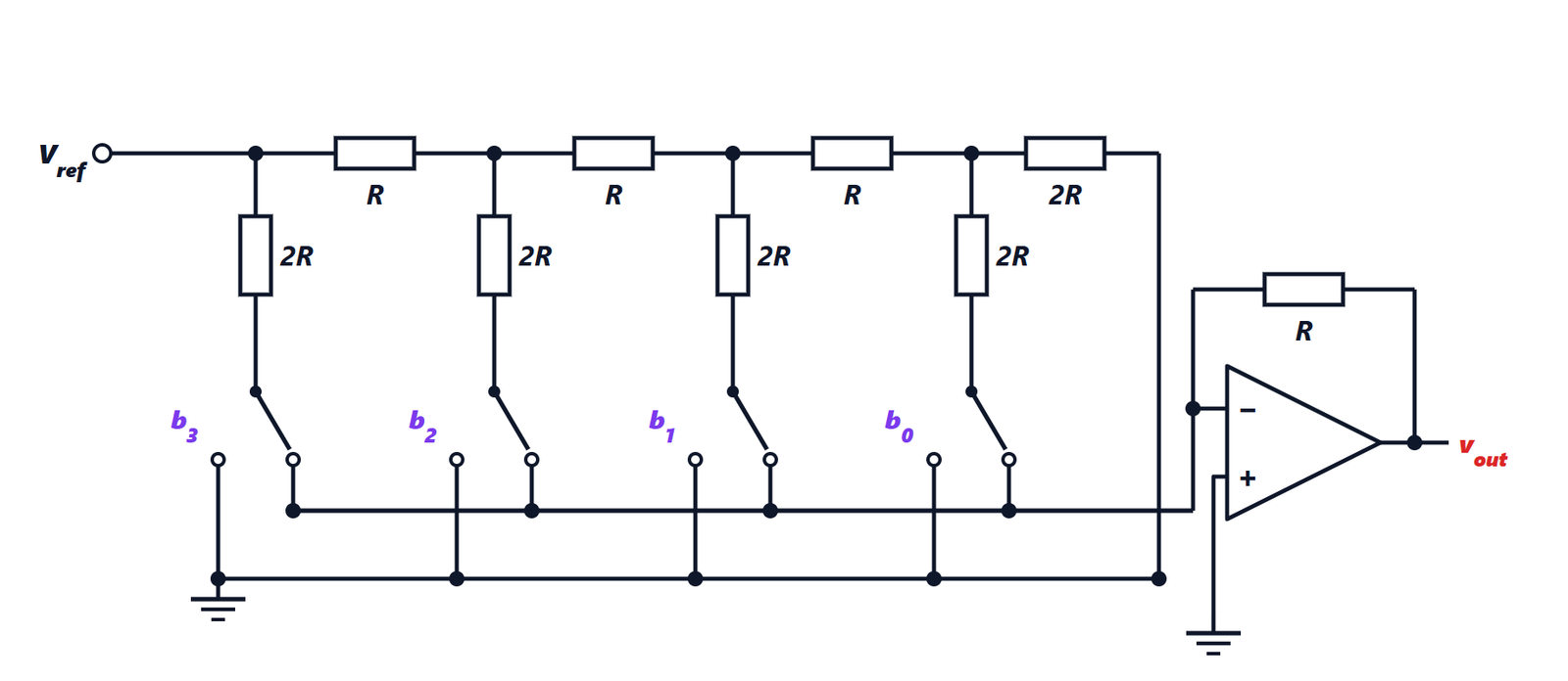
Theorem. At each node of the ladder the incoming current splits into two equal parts; the branch currents are  and the output, with feedback resistor
 , is

Proof. The switches connect each 2R branch either to ground or to virtual ground: in both cases the branch ends at zero potential, so the currents do not depend on the switch positions. Starting from the end, the last bit’s node sees to its right the  termination and below it its own branch: in parallel they make . Adding the connecting gives , and the previous node again sees two in parallel. Repeating, every node sees exactly to its right, equal to its own branch: the incoming current splits into two equal halves. The first node receives
 and sends
 into the most significant bit’s branch, the next
 , and so on. The currents of the bits at 1 enter the virtual ground and flow through the feedback resistor . ∎
Only the ratios between equal resistors matter, which an integrated circuit achieves with very high precision. With  V and 8 bits the step (LSB) is
 mV.
ADCs
Flash.  comparators compare the input with as many thresholds, in parallel: conversion takes a single cycle. Very fast (gigasamples per second), but the number of comparators doubles with every bit: it is used up to 6 to 8 bits, in oscilloscopes and radio receivers.
Successive approximation (SAR). A binary search: the converter tries the most significant bit with an internal DAC, compares with the input, keeps or discards the bit, then moves to the next. bits take comparisons. It is the most common compromise: 10 to 18 bits, from thousands to tens of millions of samples per second, low power. It is the ADC of almost every microcontroller.
A SAR conversion example. 8 bits, 5 V full scale, 3.1 V input. First step: 2.5 V (bit 7 = 1), the input is higher, the bit stays. Second: 2.5 + 1.25 = 3.75 V, too much, bit 6 goes back to 0. Third: 2.5 + 0.625 = 3.125 V, still too much, 0. Fourth: 2.5 + 0.3125 = 2.8125 V, bit 4 stays 1. Continuing down to bit 0 gives 158, that is  V, the last level below 3.1 V.
Sigma-delta. A quantiser of a few bits at a very high rate, with noise pushed to high frequencies and then filtered digitally (Signal Theory lesson on quantisation): 16 to 32 bits for audio and precision measurement, at moderate speeds.
Dual slope. The input is integrated for a fixed time, then a known reference voltage until back to zero, counting the time. Slow but very accurate and immune to 50 Hz interference if the integration time is a multiple of 20 ms: it is the converter of multimeters.
Specifications
- Resolution: the number of bits, and hence the LSB step.
- Integral nonlinearity (INL): the maximum deviation of the real characteristic from the ideal straight line, in LSB.
- Differential nonlinearity (DNL): how much each step differs from the ideal value of 1 LSB. With DNL worse than −1 LSB a code may be missing altogether; a DAC with DNL greater than −1 LSB is guaranteed monotonic (the output never falls as the code increases), an essential property in control systems.
- Effective number of bits (ENOB), derived from the measured signal-to-noise ratio (lesson on quantisation).
- Sampling rate and, for ADCs, the sample-and-hold circuit, which freezes the input during conversion: a SAR ADC needs the input to stay still for all comparisons.
A 16-bit converter with a noisy voltage reference or a disturbed ground gives fewer useful bits than a well-designed 12-bit one: accuracy depends as much on the quality of the reference, the supply and the printed circuit board as on the converter itself.