Least squares approximation and regression
The least squares problem, normal equations, calibrating a sensor, matrix form and QR, models linear in the parameters, residuals and overfitting.
Real measurements are noisy: forcing a curve through every point, as interpolation does, means following the errors too. The least squares method, invented by Gauss and Legendre in the early nineteenth century to compute planetary orbits, instead looks for the curve of a given form that passes as close as possible to all the points together. It is how sensors are calibrated, model parameters estimated and the trend line of any chart drawn.
The problem
Given  points
 , we look for a function from a chosen family, for example a line
 , that minimises the sum of the squared residuals:
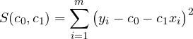
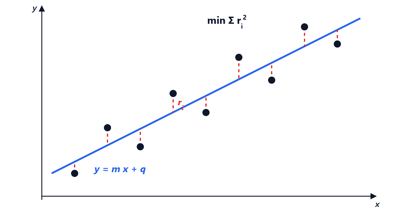
 (dashed red).
Why squares and not absolute values? Because the function to minimise becomes smooth, the minimum is found with derivatives and leads to a linear system; and because, if the measurement errors are Gaussian, the solution is also the most likely estimate of the parameters.
The normal equations
Setting the partial derivatives to zero (Analysis 2 lesson on maxima and minima):

that is
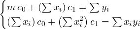
with solution

where  and
 are the means. The line always passes through the centroid of the points
 .
Example: calibrating a sensor. A temperature sensor gives the voltages 0.52, 0.71, 0.88, 1.11, 1.29 V at 0, 20, 40, 60, 80 °C. The means are  °C and
 V. The deviations from the means are
 for the temperatures and
 for the voltages, so
 and
 . The sensitivity is
 V/°C, that is 9.7 mV/°C, and the offset
 V. The model gives 0.514, 0.708, 0.902, 1.096, 1.290 V: the residuals are a few millivolts, the largest 22 mV at 40 °C.
Matrix form
The problem is written  , where
 has one row per measurement and one column per parameter (for the line, the columns are all 1s and the
 ). It is a system with more equations than unknowns, in general with no exact solution. The least squares solution satisfies the normal equations

and, as seen in Geometry and Algebra,  is the orthogonal projection of
 onto the column space of : the residual vector is perpendicular to every column.
Numerical warning. Forming  squares the condition number: if
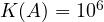 ,
 , and 12 digits are lost instead of 6. Libraries instead use the QR factorisation,
 with
 having orthonormal columns, which leads to the triangular system
 without worsening the conditioning. For the hardest problems the singular value decomposition (SVD) is used.
Not just lines
The method works with any model that is linear in the parameters, even if nonlinear in  :
- polynomials
 (of low degree, so as not to fall back into Runge’s oscillations);
- combinations of known functions, such as
 , to estimate the amplitude and phase of a signal of known frequency;
- models that become linear after a transformation:
 becomes
 . This is how the time constant of an RC discharge is estimated from a series of voltage readings.
For models that are genuinely nonlinear in the parameters (for example a diode characteristic with series resistance) iterative methods such as Gauss-Newton and Levenberg-Marquardt are used, which linearise the model at each step, just as Newton does for equations.
How good is the fit
- The residuals must show no pattern: if they form a curve, the model is wrong (for example a line fitted to quadratic data).
- The coefficient of determination
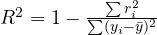 gives the fraction of variability explained by the model: 1 is perfect, 0 means the model explains nothing beyond the mean.
- Adding parameters always shrinks the residuals, but beyond a certain point the model follows the noise instead of the phenomenon (overfitting): with points, a polynomial of degree
 has zero residuals and is useless.
The same principle, minimising a squared error over a lot of data, underlies the training of neural networks: the “weights” are the parameters, and the gradient of the error guides their correction.