Inner product and orthogonality: projections, Gram-Schmidt and the spectral theorem
Inner product and norm, Pythagoras, orthogonal projection and least squares, orthonormal bases, the Gram-Schmidt process, orthogonal matrices and the spectral theorem.
Abstract vector spaces have neither lengths nor angles. To get them you need one more structure, the inner product. With it come orthogonality, projections, orthonormal bases and one of the finest theorems of the course, the spectral theorem. These are the tools behind least squares, Fourier series and JPEG compression.
Inner product and norm
An inner product on a real space  is an operation
 that gives a number and is symmetric, linear in each argument and positive definite:
 for every
 . The standard one on
 is
 . On continuous functions on
 an inner product is
 .
The norm is  , and the Cauchy-Schwarz and triangle inequalities hold (proved in the lesson on vectors, with an argument that uses only these properties). Two vectors are orthogonal if
 .
Pythagoras’ theorem
If  , then
 . In any space with an inner product, even one made of functions.
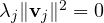
Non-zero orthogonal vectors are independent. If  , taking the inner product with
 leaves only
 , so
 .
Orthogonal projection
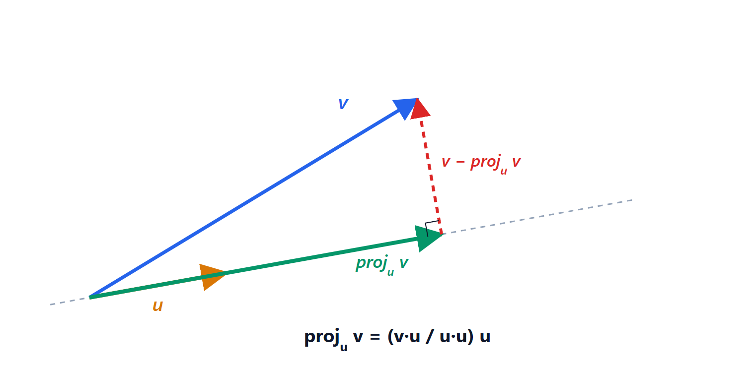
 onto the direction of
 is the vector on that line closest to . The difference
 is perpendicular to .
Proof of the formula
We look for the multiple  such that
 is orthogonal to :

It is also the closest point: for any other multiple  , the vector
 is the sum of and
 , which are orthogonal, and by Pythagoras
 .
The same holds for projection onto a subspace  : the point of closest to is the one for which the difference is orthogonal to all of . This is the principle of least squares: when a system
 has no solution (too many equations, noisy data), you look for
 such that
 is the projection of
 onto the column space. The orthogonality condition gives the normal equations
 . This is how a regression line through experimental data is computed.
Orthonormal bases
A basis is orthonormal if its vectors have norm 1 and are pairwise orthogonal. The advantage is huge: coordinates are computed with an inner product, without solving systems.
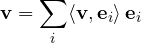
Indeed, taking the inner product of  with
 leaves only
 . A Fourier series is exactly this, in a space of functions: sines and cosines are an orthogonal basis with respect to
 , and the Fourier coefficients are inner products.
The Gram-Schmidt process
From any basis  you build an orthonormal basis of the same space by removing from each vector its projections onto the previous ones:

Example.  ,
 .
 .
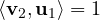 ,
 , so
 . Check:
 . Normalising:
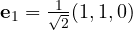 ,
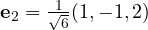 .
Orthogonal matrices
A square matrix  is orthogonal if its columns are an orthonormal basis, that is if
 . Then
 : the inverse costs as much as a transpose. Orthogonal matrices preserve inner products, lengths and angles,
 : they are the rotations (
 ) and the reflections (
 ).
The spectral theorem
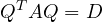
Theorem. Every real symmetric matrix has real eigenvalues and can be diagonalised with an orthonormal basis of eigenvectors: there is an orthogonal such that
A key step of the proof is easy to see: eigenvectors of distinct eigenvalues are orthogonal. If  and
 , using
 :

so  and, if
 , . You can see it in the matrix
 from the lesson on eigenvalues: its eigenvectors
 and
 are perpendicular.
The spectral theorem has consequences everywhere: the principal stress directions in a beam, the principal axes of inertia of a rigid body, principal component analysis (PCA), which reduces data to the directions of greatest variance, and the classification of conics and quadrics that we will see in the lesson on plane geometry.