Eigenvalues, eigenvectors and diagonalisation
Definition and geometric meaning, the characteristic polynomial, diagonalisation and multiplicities, uses for matrix powers, dynamical systems, circuits and Fibonacci.
A matrix transforms vectors by rotating and stretching them, but for almost every matrix there are special directions that are not rotated: vectors along those directions are just multiplied by a number. They are the eigenvectors, and the number is the eigenvalue. Finding them means choosing the frame in which the transformation becomes as simple as it gets. The idea underpins the mechanics of vibrations, the stability of control systems, data compression and even Google’s PageRank algorithm.
Definition
Let  be an
 matrix. A non-zero vector
 is an eigenvector of with eigenvalue
 if

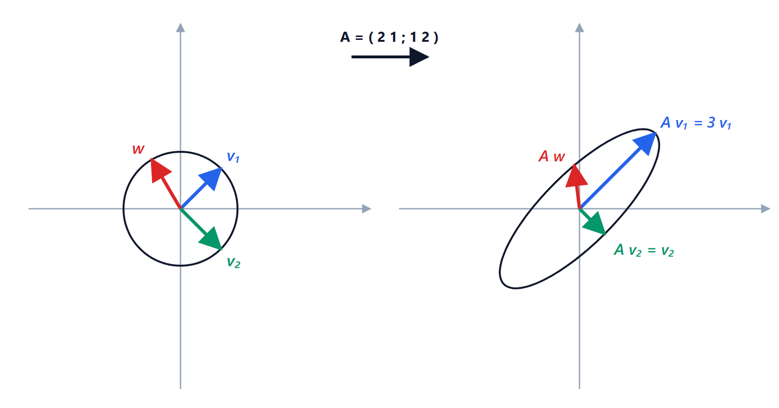
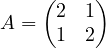 maps the circle to an ellipse. The vector
 along the diagonal is just stretched by 3,
 stays the same (eigenvalue 1); a generic vector
 changes direction. The eigenvectors are the axes of the ellipse.
The eigenvectors for the same , together with the zero vector, form a subspace, the eigenspace  .
How to find them: the characteristic polynomial
 can be rewritten as
 . This homogeneous system has a non-zero solution if and only if the matrix is not invertible, that is

 is a polynomial of degree
 , the characteristic polynomial. Its roots are the eigenvalues; for each one, the eigenvectors are found by solving .
Example. For the matrix in the figure:

 :
 gives
 , eigenvectors
 .
 :
 gives
 , eigenvectors
 .
Two useful checks: the sum of the eigenvalues is the trace (the sum of the diagonal, here  ) and their product is the determinant (
 ).
Matrices without real eigenvalues. The 90° rotation,  , has characteristic polynomial
 : no direction in the plane stays put under a rotation, and the eigenvalues are complex,
 . This is why many courses work over the complex numbers, where every polynomial has roots.
Diagonalisation
is diagonalisable if there is a basis of  made of eigenvectors. In that basis the matrix becomes diagonal, with the eigenvalues on the diagonal:
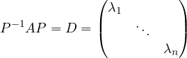
where  has the eigenvectors as columns. Indeed
 has columns
 , that is
 .
When it is diagonalisable
Eigenvectors of distinct eigenvalues are independent. We prove it for two: if  , applying gives
 ; subtracting
 times the first,
 , so
 (since
 and
 ), and then
 . For
 eigenvectors the same argument works by induction.
It follows that if has distinct real eigenvalues, it is diagonalisable. With repeated eigenvalues you need to check: for each eigenvalue the geometric multiplicity (dimension of the eigenspace) must equal the algebraic multiplicity (how many times it is a root of the polynomial). The classic counterexample is  : eigenvalue 1 twice, but only one eigenvector
 up to multiples. It is not diagonalisable.
What it is for
Matrix powers. If  , then
 , and
 is computed by raising the diagonal entries to the power. For the matrix in the figure,
 only needs
 and
 .
Discrete dynamical systems. In  the component along the eigenvector
 is multiplied by
 at every step. If every eigenvalue has modulus less than 1 the system goes to zero (it is stable); if one has modulus greater than 1 it blows up. IIR digital filters and digital controllers are designed precisely by looking at where the eigenvalues lie.
Differential equations. The system  , which describes for example an RLC circuit or two masses linked by springs, splits in the eigenvector basis into independent equations
 , with solutions
 . The eigenvalues are the “modes” of the system: for a circuit they are the poles, and their real part tells whether the circuit is stable.
Fibonacci. The sequence  can be written with the matrix
 , whose eigenvalues are
 and
 . Diagonalising gives Binet’s formula,
 , and shows why the ratio of two consecutive terms tends to the golden ratio.