Unconstrained maxima and minima: critical points, saddle points and the Hessian
Fermat's theorem, saddle points, classification with the eigenvalues and determinant of the Hessian, a complete example, absolute extrema on a compact set and least squares.
Finding the maximum or minimum of a function of several variables is the optimisation problem: the shape of a box that uses the least material, the parameters of a model that best fit some data, the weights of a neural network. In this lesson we see how critical points are found and how they are classified with the Hessian matrix.
Critical points
Fermat’s theorem. If  is differentiable and has a local maximum or minimum at an interior point
 , then

Proof. For every direction  , the one-variable function
 has a maximum or minimum at
 , so
 . A vector orthogonal to every direction is the zero vector.
Points where the gradient vanishes are called critical (or stationary): there the tangent plane is horizontal. But as in Analysis 1 the condition is only necessary: a critical point can be a maximum, a minimum, or neither.
Saddle points
In one variable, a critical point that is neither maximum nor minimum is a horizontal inflection. In two variables there is a new and very common possibility: the saddle point, where the function rises in some directions and falls in others.
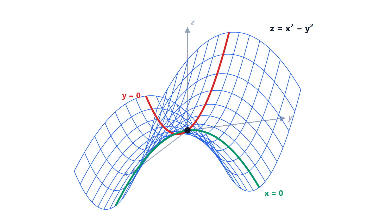
 has zero gradient at the origin, but along the
 axis (red curve) the origin is a minimum and along the
 axis (green curve) it is a maximum: it is a saddle point, like the middle of a horse saddle or a mountain pass.
Classification with the Hessian
Near a critical point, the second-order Taylor expansion reduces to its quadratic part, because the gradient is zero:

The sign of  therefore depends on the sign of the quadratic form
 . By the spectral theorem the symmetric Hessian can be diagonalised by a rotation: along the eigenvector directions the quadratic form becomes
 . So:
- all eigenvalues positive (
 positive definite): rises in every direction, local minimum;
- all negative (negative definite): local maximum;
- eigenvalues of opposite sign (indefinite): saddle point;
- some eigenvalue zero (semidefinite): the test is inconclusive, and the function must be studied another way.
The practical test in two variables
With  , the product of the eigenvalues, and
 :
 | | Point |
|---|---|---|
 | | local minimum |
|  | local maximum |
| any | saddle |
 | inconclusive |
In  variables one uses Sylvester’s criterion: is positive definite if and only if all its leading principal minors are positive.
A complete example

Critical points:  and
 . From the first
 ; substituting into the second,
 , that is
 or
 . The critical points are
 and
 .
Hessian:  ,
 ,
 .
- At :
 . Saddle.
- At :
 and
 . Local minimum, with
 .
It is not an absolute minimum: along the axis the function equals  and goes down to
 .
Absolute maxima and minima on a compact set
By Weierstrass’ theorem, a continuous function on a closed and bounded set has an absolute maximum and minimum. They can be in two places:
- at interior critical points;
- on the boundary of the set.
Compute the values at all the candidates and pick the largest and the smallest; no Hessian is needed. The boundary is studied by parametrising it (each side of a rectangle is a one-variable problem) or with the Lagrange multipliers of the next lesson.
Example.  on the square
 . The only interior critical point is
 , with
 . On the boundary: with ,
 between 0 and 1; with
 , , between 0 and 1; with
 ,
 , between 0 and 1. Absolute minimum
 at , absolute maximum
 , reached for example at the corners.
An application: the least squares line
Given experimental points  , we look for the line
 that minimises the sum of squared residuals
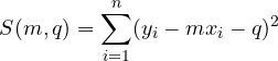
Setting  and
 gives two linear equations in
 and
 , the normal equations, and their solution is the regression line that every spreadsheet draws through data. The Hessian of
 is positive definite (if the
 are not all equal), so the critical point really is the minimum. It is the same result obtained with orthogonal projections in Geometry and Algebra, seen from the analysis side.