Flux and the theorems of Green, Gauss and Stokes
Divergence and curl, Green's theorem with proof and the planimeter, surfaces and flux, the divergence theorem, Stokes' theorem and the link with Maxwell's equations.
This lesson completes integral calculus in several variables with the three great theorems: Green, Gauss (divergence) and Stokes. They all say the same thing in different forms: the integral of a “derivative” over a region equals the integral of the function over the boundary of the region, as in the fundamental theorem of calculus. They are the language of Maxwell’s equations, and so of all of electronics.
Differential operators
For a vector field  one defines, with the symbol
 :
- the divergence
 , a scalar: it measures how much the field “flows out” of a point, like a source;
- the curl
 , a vector computed like a cross product: it measures how much the field “swirls” around a point.
The field  has divergence 3 and zero curl: it flows out of every point without swirling. The field
 has zero divergence and curl
 : it swirls around the
 axis with no sources.
Green’s theorem in the plane
Let  be a region of the plane with boundary
 traversed anticlockwise. For a field
 with continuous derivatives:

Proof (for the  part)
Let be normal with respect to the  axis:
 ,
 . Integrating first in
 :

The boundary is made of the lower curve traversed left to right, giving  , the upper curve traversed right to left, giving
 , and any vertical pieces, on which
 . The two sides match. The
 part is proved the same way with the domain normal with respect to .
Consequence: area from a boundary integral. With  ,
 the right side is the area of :

It is the principle of the planimeter, the mechanical instrument that measures an area by tracing only its outline, and of the algorithm CAD programs use to compute a polygon’s area from its vertex coordinates.
Surfaces and flux
A surface is described with two parameters,  . The vectors
 and
 are tangent, and their cross product is normal to the surface, with magnitude equal to the area of the small parallelogram
 :

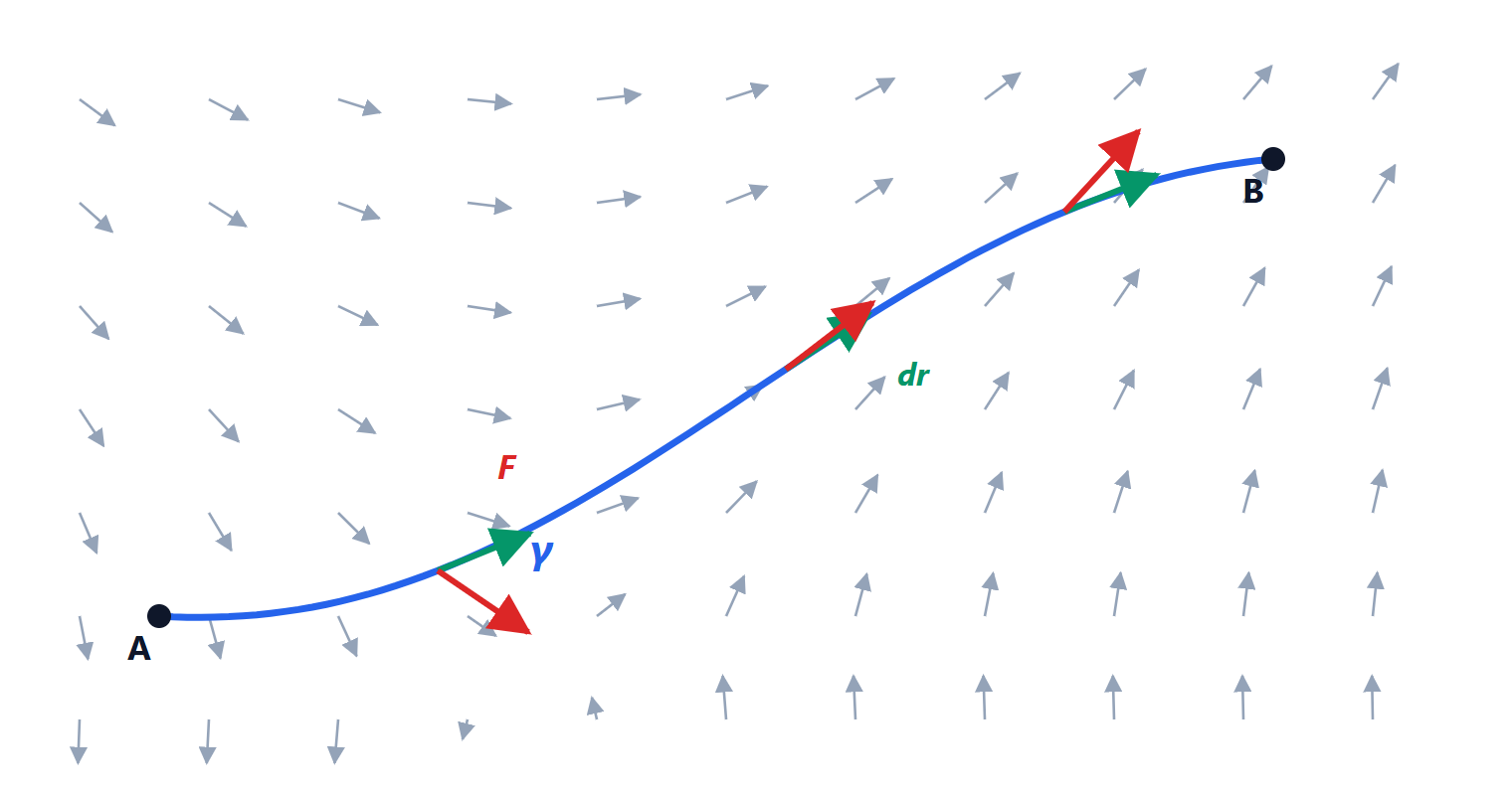
The flux of a field through an oriented surface is
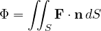
and it measures how much field crosses the surface, counting only the perpendicular component. If  is the velocity of a fluid, the flux is the flow rate, in m³/s.
Example. The flux of  through the sphere of radius
 , with outward normal: on the sphere
 , so
 and
 .
The divergence theorem (Gauss)
Let  be a solid bounded by the closed surface
 , with outward normal
 . Then

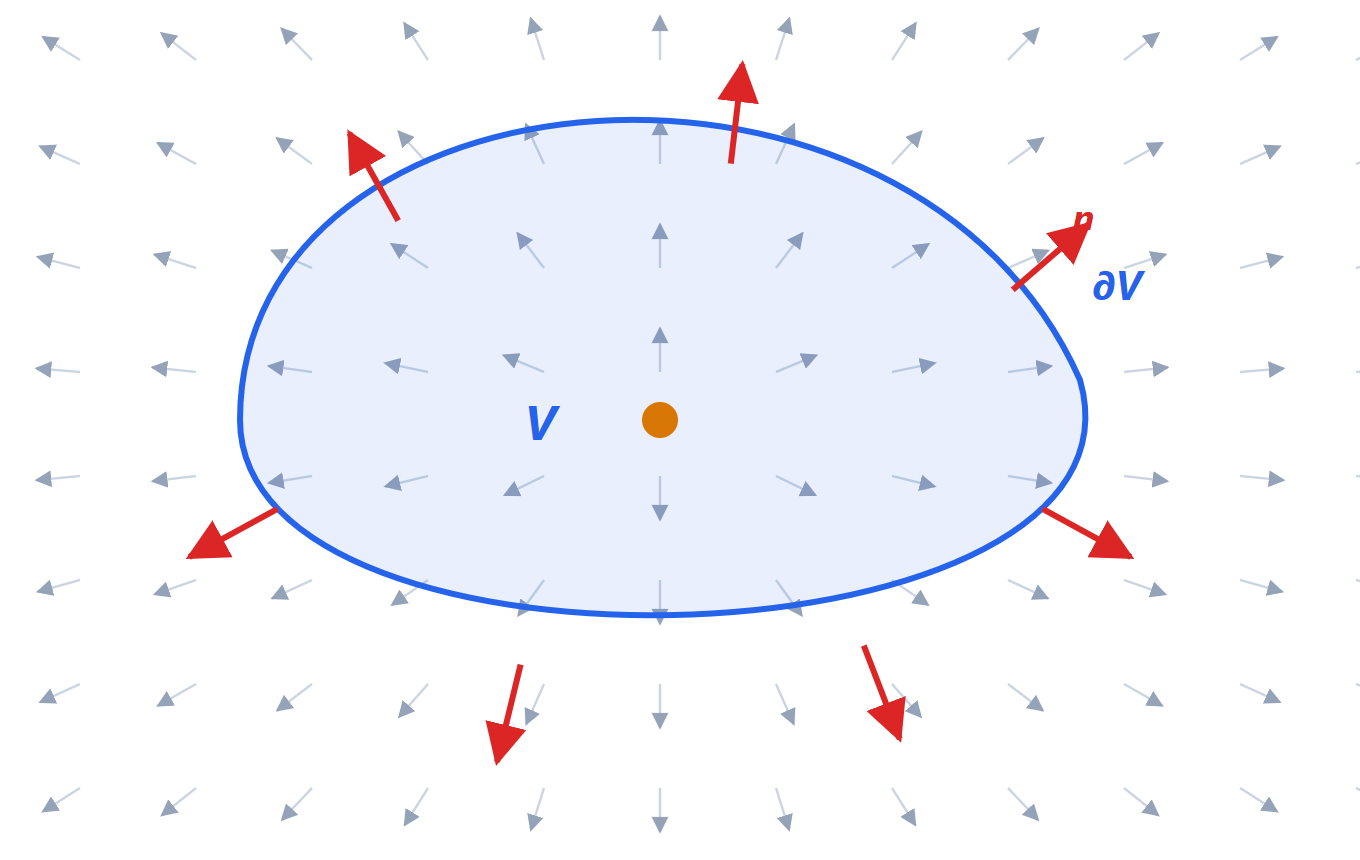 (red arrows: outward normals) equals the total of the sources inside the volume , that is the integral of the divergence. Here the field starts at a source inside and flows out everywhere.
The idea: split into many small cubes. For one cube, the outward flux computed face by face is about  times its volume. Adding over all cubes, the flux through internal faces cancels (what leaves one cube enters its neighbour) and only the flux through the outer surface remains.
Check on the example.  , and
 . It matches the flux computed directly.
In Physics 2 it becomes Gauss’s law: the flux of the electric field through a closed surface is proportional to the enclosed charge,  , and in local form
 . The divergence theorem is the bridge between the two forms.
Stokes’ theorem
Let  be a surface with boundary
 , oriented consistently (right-hand rule: with the thumb along , the fingers show the direction of the boundary). Then

The circulation of the field round the boundary equals the flux of the curl through the surface. If is flat in the  plane, it is exactly Green’s theorem. An important consequence: the flux of a curl depends only on the boundary, not on the surface chosen.
It also gives the characterisation of conservative fields from the lesson on line integrals: if  in a simply connected domain, every closed curve bounds a surface inside the domain, and the circulation is zero.
In Physics 2 it becomes Faraday’s law: the voltage induced around a loop,  , equals minus the rate of change of the magnetic flux through the loop; in local form
 . It is the working principle of transformers, generators and wireless charging.
The overall picture
| Theorem | Region | Boundary |
|---|---|---|
| fundamental theorem of calculus | segment  | two points |
| conservative fields | curve | two end points |
| Green | plane region | closed curve |
| Stokes | surface | closed curve |
| Gauss | volume | closed surface |
In every row, the integral of a derivative (gradient, curl, divergence) over the region equals the integral of the function over the boundary. In advanced mathematics all these results are a single theorem, the generalised Stokes theorem.