Double integrals: normal domains, change of variables and polar coordinates
Definition, reduction formulas and swapping the order, the Jacobian and change of variables, polar coordinates, the Gaussian integral, centres of mass and moments of inertia.
The integral of Analysis 1 computes the area under a graph. The double integral does the same one floor up: it computes the volume under a surface, but also the mass of a plate, the charge on an electrode, the centroid of a cross-section or the moment of inertia of a beam. In this lesson we see how it is defined, how it is computed by reducing it to two single integrals and how variables are changed, with polar coordinates.
The definition
Split the region  of the plane into many small rectangles of area
 , choose a point in each and form the sum
 . If, as the rectangles get smaller, the sums tend to a limit, that is the double integral:
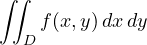
With  it is the volume of the solid between the region and the graph of
 . With
 it is the area of . Continuous functions on bounded regions with a regular boundary are always integrable, and linearity, monotonicity and additivity over regions hold.
Computing it: normal domains
The idea is to slice the solid. A region is normal with respect to the  axis if it can be described as

that is, if every vertical line cuts it in a single segment.
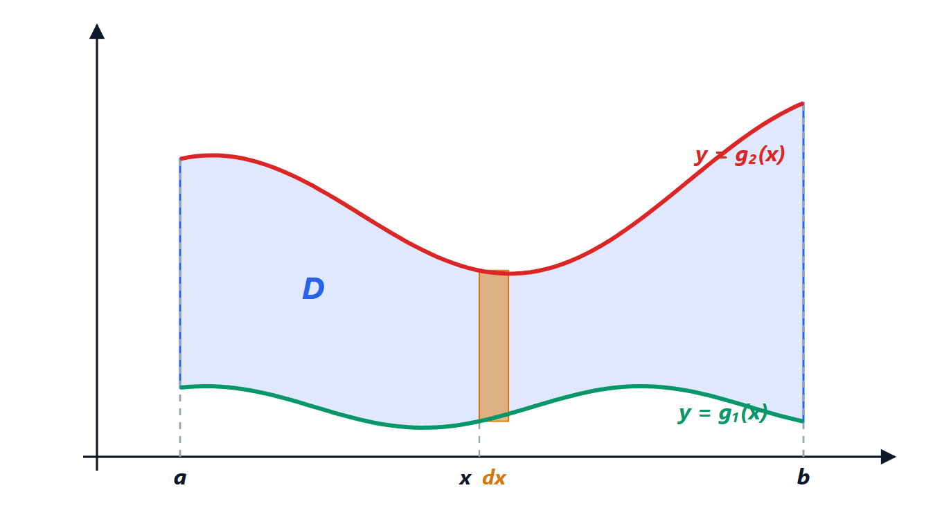 between
 and
 ,
 runs from
 to
 . The double integral is computed by first summing along the vertical strip (in ) and then adding up all the strips (in ).
Reduction formula (Fubini’s theorem):

The inner integral, with fixed, gives the area of the vertical slice; integrating the slice areas gives the volume. It is Cavalieri’s principle. In the same way you integrate first in and then in if the domain is normal with respect to the axis.
Example. 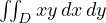 over the triangle with vertices
 ,
 ,
 , that is
 ,
 :

Swapping the order of integration
Sometimes one order leads to an impossible integral and the other to an easy one. 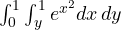 cannot be computed as it stands, because
 has no elementary antiderivative. The domain is the same triangle as before, seen as , . Swapping:

Change of variables
Switching to new variables  with
 ,
 , the small rectangles
 become curved parallelograms of area
 , where
 is the Jacobian matrix of the transformation. It is the determinant as the area scaling factor, seen in Geometry and Algebra:

Polar coordinates
With  ,
 :


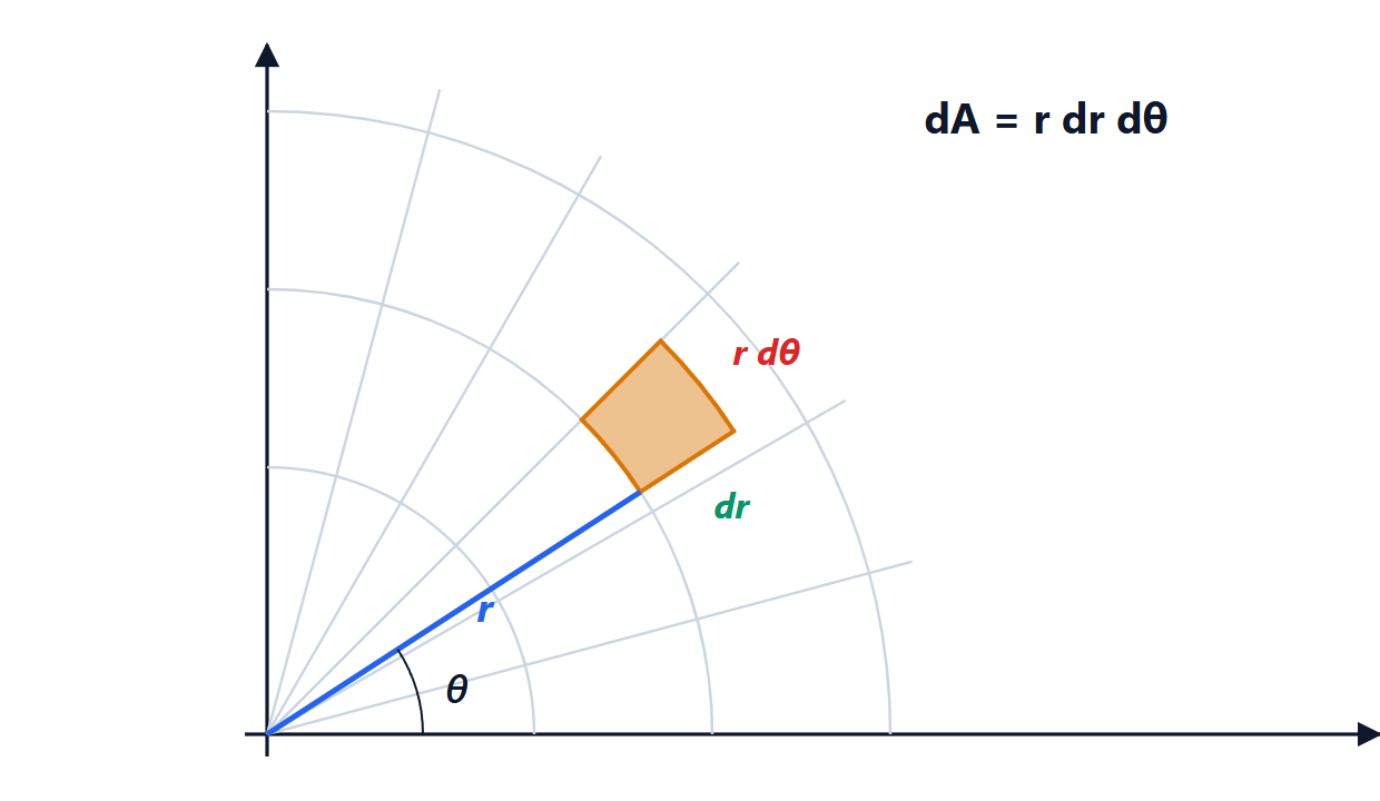
 and
 : its area is
 . The factor
 explains why regions far from the origin weigh more.
Polar coordinates simplify everything with circular symmetry: discs, annuli, sectors, and functions depending on  .
Example: the area of a circle.  .
The Gaussian integral
 cannot be computed with antiderivatives. The trick is to square it and move to the plane:

so  . It is the result that normalises the Gaussian distribution, used everywhere from statistics to thermal noise in circuits.
Physical applications
For a plate with surface density  :
- mass
 ;
- centre of mass
 ,
 ;
- moment of inertia about the origin
 .
Example. The moment of inertia of a uniform disc of mass  and radius
 (density
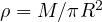 ):
 . It is the value in the table of the Physics 1 lesson on the rigid body, now proved.