Ordinary differential equations: first order and second-order linear
Direction fields and existence and uniqueness, separable equations, first-order linear equations and the RC circuit, second order with constant coefficients, RLC and resonance.
A differential equation links an unknown function to its derivatives. It is the natural way of writing the laws of physics, which say how things change: Newton’s second law, the charging of a capacitor, the cooling of a component, the growth of a population. In this lesson we cover the most important first-order equations, the existence and uniqueness theorem, and second-order linear equations with constant coefficients, which describe oscillators and RLC circuits.
Definitions
An ordinary differential equation of order  links
 to its derivatives up to
 . An initial value problem (Cauchy problem) adds initial conditions: for first order the value
 , for second order also the derivative
 .
The geometric meaning
A first-order equation  assigns a slope to every point of the plane. Drawing a short dash with that slope at many points gives the direction field, and the solutions are the curves that follow the dashes.
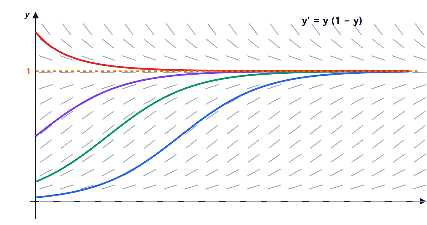
 and four solutions with different initial conditions. All those starting with
 tend to the equilibrium
 : those below rise with the typical S shape, the one above comes down.
Existence and uniqueness theorem (Picard-Lindelöf). If  is continuous and has a continuous derivative
 near
 , the initial value problem has exactly one solution near
 . Geometrically: exactly one solution curve passes through each point, and two different solutions never cross. In the figure the solutions never cross the line , which is itself a solution.
Separable equations
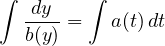
They have the form  . If
 , the constant
 is a solution. Otherwise separate the variables and integrate:
Example: Newton’s law of cooling. A heat sink at temperature  in surroundings at
 cools as
 . Separating:
 , so

The temperature difference halves every  seconds, the same exponential law as a capacitor discharging.
Example: the logistic equation in the figure, . Separating with partial fractions,  , gives
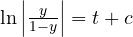 and
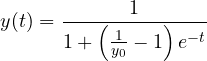
It is the model of growth that slows as resources run out: populations, the spread of a product on the market, epidemics.
First-order linear equations

Proof of the solution formula
Let  be an antiderivative of
 . Multiplying by the integrating factor
 , the left side becomes the derivative of a product:

Integrating:

Example: charging a capacitor. In an RC circuit driven by a voltage step  , the capacitor voltage satisfies
 . With
 ,
 ,
 :

Starting from empty, after a time  the capacitor is at 63% of , after
 at more than 99%.
Second-order linear equations with constant coefficients

As for linear systems (the Geometry and Algebra lesson on Rouché-Capelli), the general solution is one particular solution plus the general solution of the homogeneous equation. The solutions of the homogeneous equation form a vector space of dimension 2.
The homogeneous equation: the characteristic equation
Looking for solutions of the form  gives
 . Three cases:
| Roots | General solution of the homogeneous equation |
|---|---|
distinct real  |  |
repeated real  |  |
complex  |  |
The complex case follows from Euler’s formula:  , and the real and imaginary parts are two independent real solutions.
Example: the series RLC circuit with no source,  . The characteristic equation has discriminant
 :
 : negative real roots, the charge decays without oscillating (overdamped);
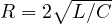 : a repeated root, the fastest return without oscillation (critically damped);
 : complex roots, a damped oscillation with angular frequency
 (underdamped).
They are the same three regimes as the pendulum with friction in the Physics 1 lesson on oscillations: the same equation, with the same solutions.
The particular solution
For forcing terms  that are polynomials, exponentials, sines or cosines, use the method of undetermined coefficients: try a solution of the same form with coefficients to be found. If that form matches a solution of the homogeneous equation (resonance), multiply it by
 .
Example.  . The homogeneous equation has solutions
 . Try
 :
 ,
 . General solution:
 . If instead the forcing were
 , at the system’s own natural frequency, you would have to try
 : the amplitude grows linearly in time, which is undamped resonance.
Beyond: systems and numerical methods
An equation of order is equivalent to a system of first-order equations,  , which in the constant-coefficient case is solved with the eigenvalues of
 , as seen in Geometry and Algebra. When there is no closed-form solution, numerical methods are used: Euler’s method (
 ) follows the direction field in small steps, and Runge-Kutta methods do the same with far more accuracy. It is what SPICE does when it simulates a circuit in time.