State-space representation, equilibria and linearisation
The concept of state, classification of systems, linear time-invariant systems, an RLC circuit example, equilibrium points, linearisation with proof, the pendulum, changes of coordinates.
Systems theory studies in a unified way very different objects, circuits, machines, chemical reactions, populations, economies, looking only at how causes (inputs) produce effects (outputs) over time. Its central tool is the state-space representation. In this lesson we look at what the state is, how systems are classified, equilibrium points, linearisation with its proof and the example of the pendulum, and changes of coordinates.
The state
A dynamical system has memory: the output at an instant depends not only on the input at that instant, but on the whole past history. The state  is the minimal information about the past that, together with the future input, determines the whole future evolution. In an electric circuit it is the voltages across capacitors and the currents in inductors; in a mechanical system the positions and velocities; in a tank the levels.
The continuous-time input-state-output representation is

with  (the number
 is the order of the system), input
 and output
 . The first is the state equation, the second the output map. In discrete time the derivative is replaced by the next step,
 .
Classification
- Linear if
 and
 are linear in
 and
 ; superposition then holds.
- Time-invariant if and do not depend explicitly on time.
- Strictly proper if the output depends on the input only through the state, i.e. there is no instantaneous link.
The most studied case, and the basis of the whole course, is the linear time-invariant system:

with constant matrices  (
 ),
 (
 ),
 (
 ) and
 (
 ).
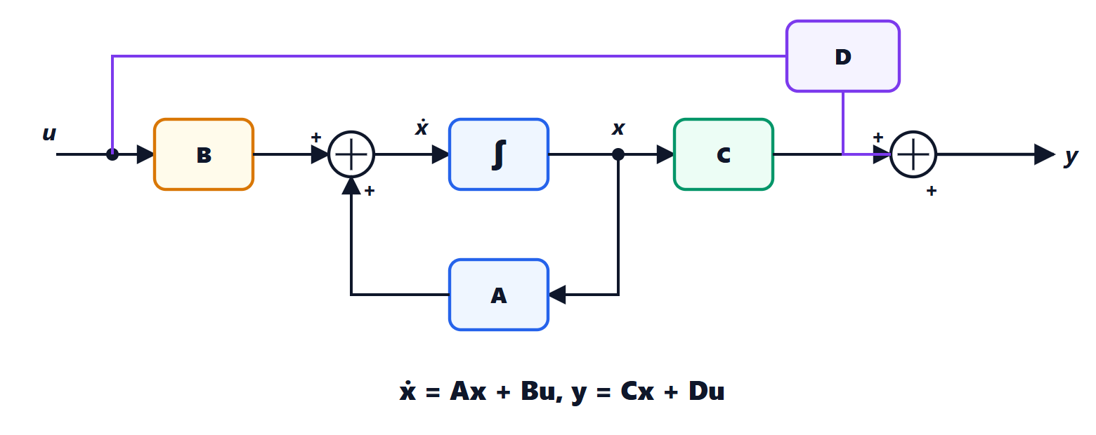
Example: a series RLC circuit. With state  (capacitor voltage) and
 (inductor current), input the source voltage and output
 :

i.e. 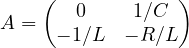 ,
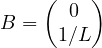 ,
 ,
 .
Equilibrium points
With a constant input  , a state
 is an equilibrium if, starting there, the system stays there:
 . A linear system with invertible has a single equilibrium,
 ; a non-linear system can have many, of different nature.
Linearisation
Almost all real systems are non-linear, but around an equilibrium they behave like a linear system.
Theorem. Let  be an equilibrium of
 with differentiable . For small deviations
 ,
 , to first order,

Proof. Since is constant,  . The first-order Taylor expansion around
 gives

and the first term is zero because the point is an equilibrium. Neglecting the higher-order terms, the linear system remains. ∎
The matrices and are the Jacobians of . The output is linearised in the same way, with  and
 .
The example of the pendulum
A pendulum of length  , with viscous friction and an applied torque , with state
 (angle from the downward vertical) and
 :

With  the equilibria are
 ,
 : the pendulum hanging down (
 ) and the inverted pendulum (
 ). The Jacobians are

because the derivative of  is
 , which is
 at 0 and
 at
 . The two matrices differ by a sign, and that sign decides everything: the first describes damped oscillations, the second an unstable system (lesson on stability). It is the same model as the inverted pendulum on a cart and the Segway, which stay upright only thanks to feedback.
Changes of coordinates
The state is not unique: if  is an invertible matrix,
 is also a state. Substituting
 :

The two representations describe the same system: they have the same eigenvalues (the matrices and  are similar) and the same input-output relation. Choosing well gives more convenient forms, such as the diagonal one, in which each coordinate evolves on its own, or the canonical forms (lesson on realisation).





