Observability, duality and the Kalman decomposition
The observability test with proof, the tanks-in-series example, the duality principle, the Kalman decomposition into four parts, transfer function and minimal realisations, detectability.
The state of a system is almost never measured in full: some outputs are measured. The question symmetric to reachability is: by watching the output (and knowing the input) for some time, can the state be reconstructed? This is observability. In this lesson we look at Kalman’s observability test with proof, the duality principle, the Kalman decomposition into four parts and the very important fact that the transfer function sees only the reachable and observable part.
Definition and test
The system is observable if, given the input and the output over a finite interval, the initial state  is uniquely determined. Since the contribution of the input to the output can be computed (it is the forced response), it is enough to study the free response: the question is whether two different initial states can give the same free output. Define the observability matrix
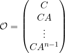
Theorem. The system  ,
 is observable if and only if
 . In that case
 output samples are enough.
Proof. The free output is  . Collecting the first samples:
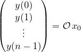
The linear system in has a unique solution if and only if  has rank . Further samples do not help: by Cayley-Hamilton
 with
 is a combination of rows already present. If the rank is less than , every in the kernel of gives an identically zero output, and cannot be told apart from zero. ∎
In continuous time the test is the same: the derivatives  at
 equal
 , and the reasoning is identical (or uses the observability Gramian). The kernel of is the unobservable subspace: the states that “cannot be seen” from the output.
Example. The two tanks in series of the lesson on reachability, 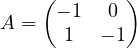 . If the first is measured,
 , then
 : has rank 1, and the level of the second is invisible, because it does not affect the first. If the second is measured,
 ,
 : rank 2. The second tank “carries” information about the first, because the first feeds it. In general, what lies upstream of the sensor is well observed.
Duality
Comparing the two matrices:  , which is the reachability matrix of the system with matrices
 and
 in place of
 and
 .
Theorem (duality). The pair  is observable if and only if the pair
 is reachable.
Proof. A matrix and its transpose have the same rank, and  . ∎
Every result on reachability therefore translates into one on observability. In particular, just as reachability allows the eigenvalues to be assigned with state feedback, observability allows those of an observer, which estimates the state from the measurements, to be assigned (Automatic Control lesson on state space); designing one is designing the other on the dual system.
The Kalman decomposition
Combining the two properties, with a suitable change of coordinates the state splits into four parts:
- RO: reachable and observable;
- RŌ: reachable but not observable;
- R̄O: not reachable but observable;
- R̄Ō: neither reachable nor observable.
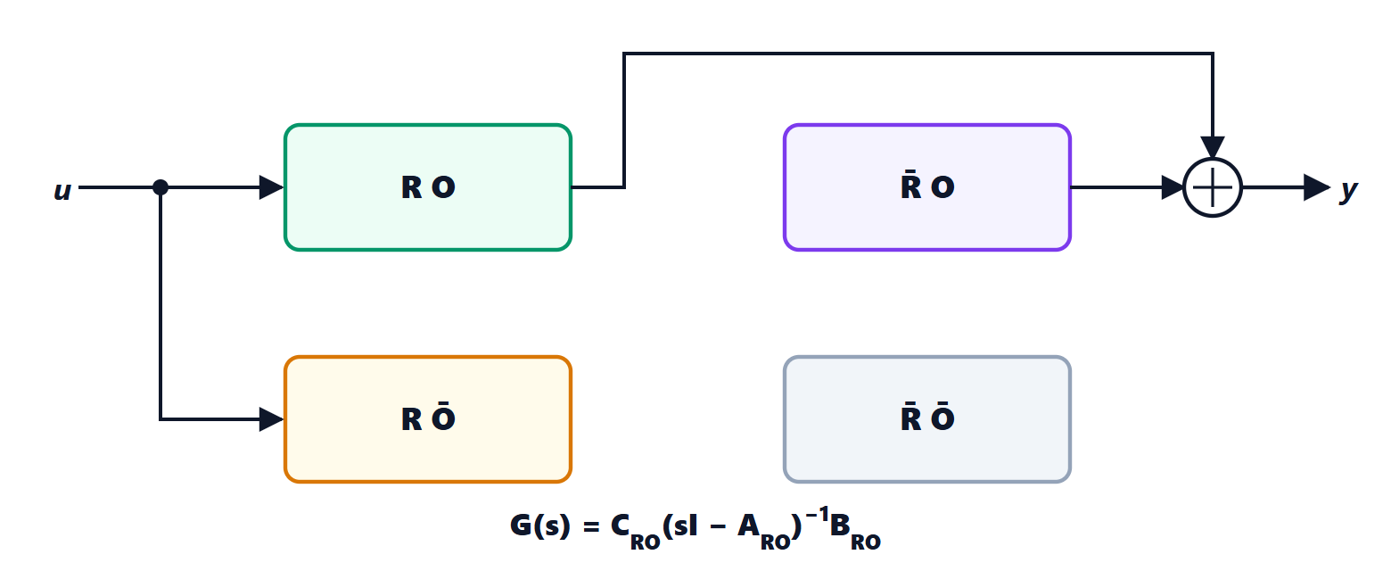
Theorem. The transfer function depends only on the reachable and observable part:

Idea of the proof. In Kalman coordinates the matrix is block triangular, has zero components on the unreachable parts and  has zero components on the unobservable parts. The inverse of a block-triangular matrix is block triangular with the diagonal blocks inverted, and in the product
 the zeros of and eliminate every term except that of the RO block. ∎
The consequences are far-reaching:
- the eigenvalues of the other three parts do not appear as poles of
 : they have cancelled with zeros. This is why the system in the example of the lesson on stability was BIBO stable but internally unstable;
- a transfer function of order
 describes a system with at least states; a representation with exactly states is called minimal, and it is minimal if and only if it is reachable and observable;
- a hidden unstable mode (unreachable or unobservable) cannot be corrected by any controller using that input and that output: it must be fixed by changing actuators or sensors.
A system is called detectable if all its unobservable modes are asymptotically stable: it is the condition, dual to stabilisability, needed to build an observer whose error tends to zero.