Non-linear systems: phase portrait and Lyapunov's methods
Multiple equilibria, limit cycles, finite escape time and chaos, the pendulum phase portrait, the indirect method, Lyapunov's direct method with proof, pendulum energy, LaSalle's principle.
Linear systems are a mathematical convenience: almost everything in the real world is non-linear, starting with the saturation of every actuator. Non-linear systems can do things linear ones cannot: have several equilibria, oscillate with a fixed amplitude independent of the initial conditions, blow up in finite time, behave chaotically. In this lesson we look at these phenomena, the phase portrait, Lyapunov’s indirect method (linearisation) and the direct method, with the proof of the theorem and the example of the pendulum, in which energy is the Lyapunov function.
Phenomena that linear systems do not have
- Several isolated equilibria. A linear system has a single equilibrium, or infinitely many on a subspace; the pendulum has two of opposite nature, hanging down and inverted (and their copies every
 ).
- Limit cycles. An isolated oscillation, with its own amplitude and period, towards which nearby trajectories converge. The Van der Pol oscillator,
 , has negative damping at small amplitudes and positive damping at large ones: small oscillations grow, large ones decay, and everything converges to the same cycle. It is the working principle of electronic oscillators, in which the amplifier’s non-linearity sets the amplitude (Applied Electronics lesson on oscillators).
- Finite escape time. The equation
 with
 has solution
 , as can be checked by differentiating: it goes to infinity at the instant
 . No linear system does this: at most it grows exponentially.
- Chaos. Already with three states, deterministic systems such as the Lorenz equations have bounded but long-term unpredictable trajectories, because tiny errors in the initial condition grow exponentially.
The phase portrait
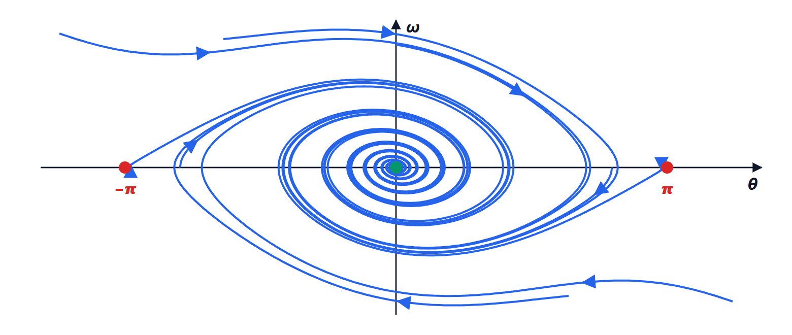
For second-order systems the trajectories are drawn in the state plane: the phase portrait. It shows equilibria, regions of attraction and cycles at a glance.
The indirect method: linearisation
Theorem (Lyapunov’s indirect method). Let  be the Jacobian of the system at an equilibrium (lesson on representations).
- If all the eigenvalues of have negative real part, the equilibrium is locally asymptotically stable.
- If at least one eigenvalue has positive real part, the equilibrium is unstable.
- If the eigenvalues have non-positive real part and some lie on the imaginary axis, linearisation says nothing: the non-linear terms decide.
The idea of the proof is to use as a Lyapunov function for the non-linear system the quadratic function  found for the linearised system (lesson on stability): close to the equilibrium the non-linear terms are of higher order and cannot change the sign of its derivative.
Example. For the pendulum with friction, the characteristic polynomial of the Jacobian is  at the bottom, with roots of negative real part: stable. At the inverted equilibrium it is
 , whose negative constant term guarantees a positive real root: unstable, a saddle point.
The critical case is not rare. Without friction ( ) the eigenvalues at the bottom are
 , on the imaginary axis, and linearisation cannot decide. The direct method is needed.
Lyapunov’s direct method
Theorem. Let the origin be an equilibrium of  and let
 be a continuously differentiable function, positive definite in a neighbourhood of the origin (
 ,
 elsewhere). If along trajectories
 , the origin is stable. If
 for every
 , it is asymptotically stable.
Proof (stability). Given  , let
 be the minimum of on the sphere
 , positive because is positive definite. The set
 contains the origin and, by continuity of , a ball of radius
 around it. A trajectory starting in this ball has
 at the start, and since does not increase, it keeps forever. To leave the ball of radius
 it would have to cross its surface, where
 : impossible. So it stays within . ∎
The method does not require solving the equations, and it works far from the equilibrium. The difficulty is finding : there is no general recipe, but for physical systems energy is the first candidate.
The example of the pendulum
For the pendulum  ,
 , take the mechanical energy per unit mass, kinetic plus potential (divided by
 ):

It is positive definite near the origin ( for
 ). Its derivative along trajectories is

So the downward equilibrium is stable, even without friction, where  and energy is conserved: the case linearisation could not decide. With friction
 is only negative semidefinite (it is zero when
 , whatever
 ), so the theorem gives only stability. LaSalle’s invariance principle completes the reasoning: trajectories converge to the largest invariant set contained in
 ; but if
 stays zero,
 must also be zero, and near the origin this happens only for
 . The equilibrium is therefore asymptotically stable, as the phase portrait shows.
Beyond analysis
The same ideas are used for design. The control of a Segway or of an inverted pendulum on a cart is usually designed on the model linearised around the upright position, and works as long as the angle stays small. For large excursions non-linear techniques are used: feedback linearisation, which cancels known non-linearities with the command itself; variable-structure control (sliding mode), robust to uncertainties; and direct design of controllers that make the derivative of a Lyapunov function chosen in advance negative.