Realisation: canonical forms, modal form and cancellations
The realisation problem, the controllable canonical form with proof, the companion matrix, reachability proved, the observable form by duality, the modal form from partial fractions, cancellations and hidden modes.
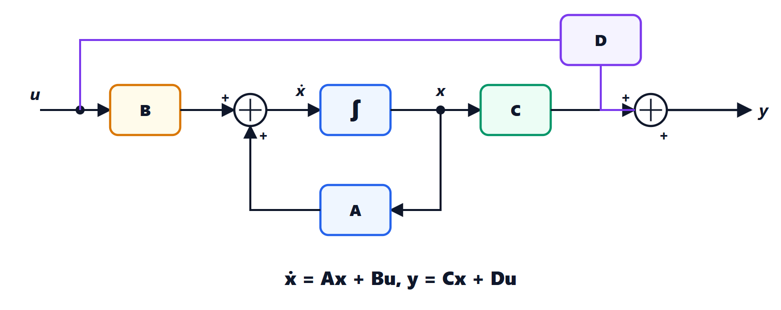
Often what is known about a system is its transfer function, obtained from measurements or from a frequency-domain design, and a state-space representation is needed: to simulate it, to implement it in a circuit or a program, to design state feedback. This is the realisation problem. In this lesson we look at the controllable canonical form with proof, why it is always reachable and when it is observable, the dual form, the modal form from partial fractions, and what happens when there are cancellations.
The problem
Given a rational transfer function  , we look for
 such that
 . If
 is proper but not strictly (numerator and denominator of the same degree), divide first:
 and realise the strictly proper remainder. There are infinitely many realisations, because every change of coordinates produces another one (lesson on representations); the most useful ones are the canonical forms.
The controllable canonical form
Consider, to fix ideas, a third-order system:

Theorem. A realisation of is

Proof. Introduce an auxiliary variable  defined by
 , i.e.
 . Then
 , i.e.
 . Choosing as state
 ,
 ,
 gives
 ,
 and, from the differential equation,
 : these are the rows of
 and
 . The output
 gives
 . ∎
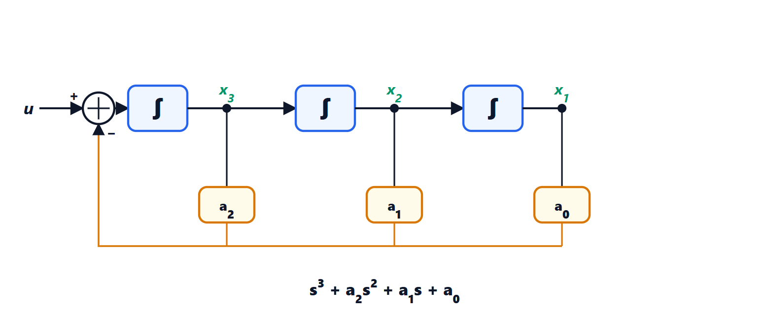
The matrix is called a companion matrix: the coefficients of its characteristic polynomial are exactly the  of the last row. The realisation is also a practical recipe: a chain of
 integrators with constant feedbacks, as was done with analogue computers and as one writes in a simulation program.
Theorem. The controllable canonical form is always reachable.
Proof. Compute  :
 ,
 is the last column of ,
 , and
 . The matrix
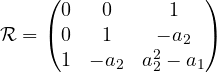
is triangular with respect to the anti-diagonal with all 1s on it, so it has determinant  and full rank, whatever the coefficients. ∎
Observability, instead, is not guaranteed: the controllable canonical form is observable if and only if numerator and denominator have no common roots. If there is a cancellation, the realisation has more states than needed, and the extra part is unobservable.
The dual form
Transposing the controllable canonical form ( , with
 in place of and
 in place of ) gives the observable canonical form. The transfer function does not change, because is a scalar and equals its transpose:
 . By duality (lesson on observability) this form is always observable, and it is reachable only if there are no cancellations.
The modal form
If the poles  are distinct, the partial fraction expansion
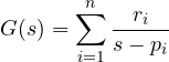
immediately suggests a diagonal realisation:  for each
 , and
 . Each state is a mode, and the subsystems work in parallel. Every mode is reachable (the input enters all of them) and observable if and only if its residue
 is non-zero: a zero residue is exactly a cancelled pole.
Example. For  the residues are
 and
 , so

The controllable canonical form of the same function has 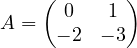 (the matrix of the example in the lesson on the solution),
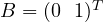 and
 . The two realisations are related by a change of coordinates, the one that diagonalises .
Cancellations
Change the numerator to  :
 . The canonical form with
 has two states and is reachable, but the transfer function is first order: the realisation is not minimal, and by the theorem of the lesson on observability the extra part must be unobservable. Indeed
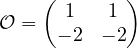 has rank 1. The mode
 is there, but the output does not see it.
Here the hidden mode is stable and does no harm. If it were unstable, and the system were actually built that way (in a circuit, or as the series of a controller and a process), we would have a system that looks perfect from its transfer function and yet diverges. The moral of realisation theory: the transfer function describes the input-output behaviour, not the system; to know everything one needs the state-space representation, or the certainty that it is minimal.