Transmission lines: the telegrapher's equations and characteristic impedance
When the line model is needed, distributed parameters, the telegrapher's equations with proof, waves and characteristic impedance, coaxial cable, losses and reflections in time.
In Electrical Engineering circuits we assume that the voltage at a node is the same at every point of the wires forming it. This holds as long as the wires are much shorter than the wavelength. When they are not, a voltage change takes a noticeable time to travel along them, and the connection must be treated as a transmission line: coaxial cables, twisted pairs, fast printed circuit traces, power lines hundreds of kilometres long. In this lesson we derive the line equations and the meaning of the characteristic impedance.
When the line model is needed
The rule of thumb: if the length of the connection exceeds about a tenth of the wavelength, propagation must be taken into account.
- At 50 Hz
 km: only very long power lines are transmission lines.
- At 1 GHz
 cm in vacuum and about 15 cm in a printed circuit board: any trace a few centimetres long is one.
- In digital circuits the edge rise time is what counts: with 1 ns edges the signal travels about 15 cm of trace during the rise, so traces longer than a few centimetres must be designed as lines.
The distributed-parameter model
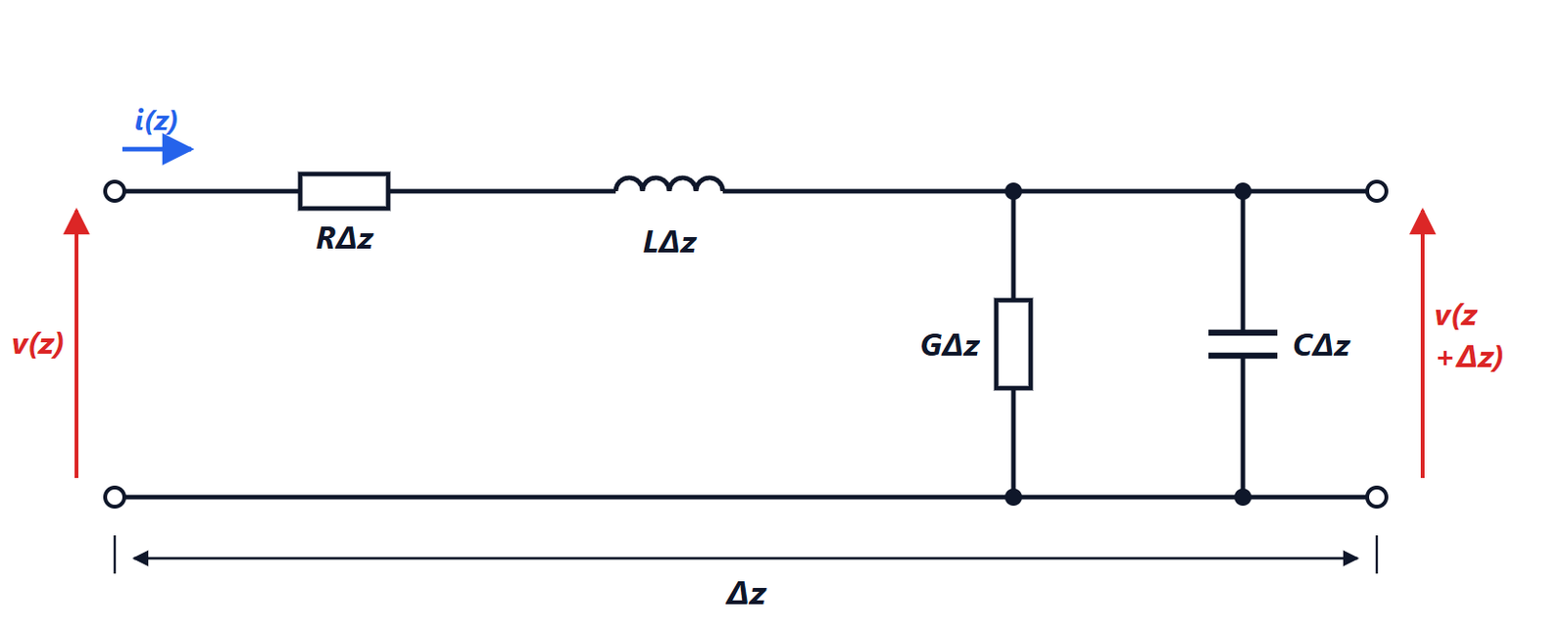
A line is made of two conductors. A section of length  is represented by a series resistance and inductance (the conductors) and a shunt conductance and capacitance (the insulation between them), all proportional to :
 are the per-unit-length parameters.
The telegrapher’s equations
Theorem. Voltage and current along the line satisfy

Proof. Apply Kirchhoff’s voltage law to the section:  . The current law at the right-hand node:
 (up to terms of order
 ). Dividing by and letting it go to zero gives the two equations. ∎
Waves on the line
In sinusoidal steady state, with phasors  and
 :

Differentiating the first and substituting the second,  , with the propagation constant

The general solution is the sum of a wave going towards  and one coming back:

where the current expression follows from the first equation, with
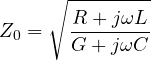
the characteristic impedance: the ratio of voltage to current of a wave travelling in one direction only.
The lossless line
With  , a good approximation for sections that are not too long:

 is real and independent of frequency. Careful: it is not a resistance that dissipates, but the ratio
 an infinitely long line would present to the source, while the energy travels away and never comes back.
Example. A coaxial cable with  nH/m and
 pF/m has
 Ω and
 m/s, two thirds of the speed of light: one metre of cable delays the signal by 5 ns.
The coax. For conductors of diameter  (inner) and
 (outer) separated by a dielectric of relative permittivity
 , the Physics 2 formulas for capacitance and inductance give
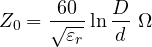
The common RG-58 ( mm,
 mm, polyethylene with
 ) gives about 50 Ω. The standard values are 50 Ω for radio frequencies (a compromise between power handling and losses) and 75 Ω for television (minimum loss).
In every line where the field is transverse (TEM),  : the velocity is that of light in the dielectric,
 , whatever the geometry.
Lossy lines
Losses attenuate the wave by  , and are expressed in dB per metre or per 100 m. They grow with frequency: the resistance
 grows as
 because of the skin effect, and dielectric losses (
 ) in proportion to
 . An observation by Heaviside: if
 ,
 and do not depend on frequency and the line, although it attenuates, does not distort. In early twentieth-century telephone lines inductors were added along the cable (loading coils) precisely to approach this condition.
Reflections in time
If a voltage step travels along a line and reaches an end terminated in , it is completely absorbed. If the end is open or short-circuited, or terminated in a different load, part of it comes back: for a digital circuit this means ringing and false edges. That is why the lines of fast buses (USB, HDMI, Ethernet, computer memory) are designed with controlled impedance and terminated in the characteristic impedance. Reflection is also used as a tool: the time-domain reflectometer (TDR) sends a pulse into the cable and from the delay of the echo computes where a fault is, to within centimetres.