The printed circuit board: return current, ground plane and decoupling
Distribution of the return current under the trace and the fraction within a distance proved, slots and layer changes, decoupling capacitor resonance, layer stack-up.
A device’s electromagnetic compatibility is decided largely on the printed circuit board: that is where the radiating loops arise, the ground drops that drive common-mode currents, the current peaks of the supplies. The rules of good layout follow almost entirely from one principle: current returns wherever it can with the lowest impedance, and at high frequencies this means directly under the trace. In this lesson we look at the distribution of return current in a ground plane with the calculation of the fraction concentrated under the trace, the mistakes that interrupt it, supply decoupling with its resonance, and the choice of layer stack-up.
Where the current returns
At low frequency the return current in the ground plane distributes according to resistance, i.e. along the shortest path between the two ends. But above a few tens of kilohertz inductance dominates, and the current chooses the path that minimises the area of the loop formed with the outgoing current, because inductance is proportional to the linked flux (Physics 2 lesson on inductance). The minimum-area path is right under the trace.
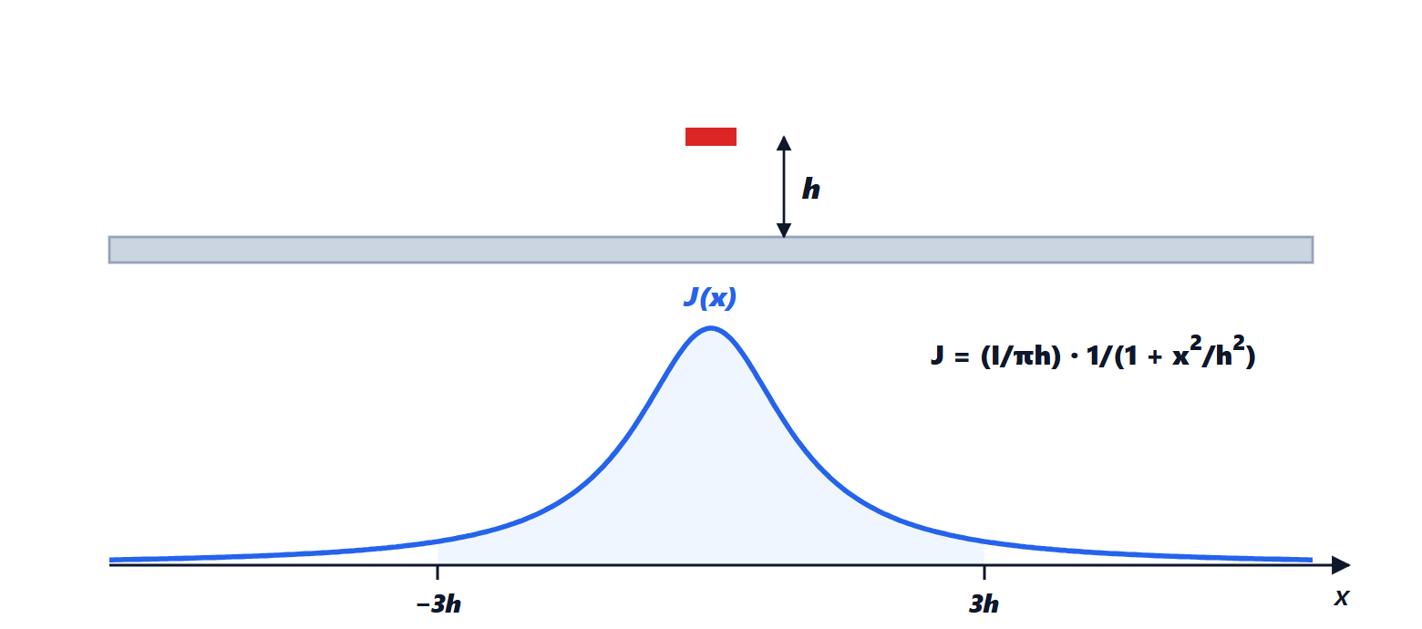
For a thin trace at height  above a very large conducting plane, the return current density (per unit width) at a distance
 from the trace’s vertical is
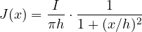
(obtained with the method of images: the plane is equivalent to an image wire at depth , and the current in the plane is the one that cancels the tangential magnetic field below the plane).
Theorem. The total current in the plane is  , and the fraction flowing within distance
 of the trace’s vertical is
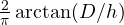 .
Proof. With the substitution  :

For  the arctangent tends to
 and we get : all the current returns. ∎
Example. Within  flows
 % of the current; within
 , about 94 %. With traces 0.1 mm above the plane, almost all the return current lies in a strip a couple of millimetres wide under the trace.
Mistakes that interrupt the return
The return current needs that strip. If it is interrupted, the current must go around the obstacle, the loop widens and the trace becomes an antenna (lesson on radiated emissions):
- slots in the ground plane: a trace crossing a slot forces the current to go around it. It is the most common mistake, often caused by a row of closely spaced vias or by a plane split into “analogue” and “digital” areas;
- layer changes: if a trace moves from a layer referenced to the ground plane to one referenced to the supply plane, the return must jump between planes; a capacitor or a ground via near the change is needed;
- traces at the board edge: half of the distribution is missing, and the field escapes outwards.
A single continuous ground plane is almost always the best choice even for mixed-signal circuits: it is enough to place the components so that digital currents do not flow under analogue circuits. The star ground remains useful for large low-frequency currents (lesson on coupling).
Supply decoupling
When an integrated circuit switches, it draws current peaks in nanoseconds. If they had to come from the power supply through long traces, their inductance would produce voltage drops and large current loops. Decoupling capacitors close to the supply pins provide the charge locally, and the loop of the peaks closes between capacitor and component.
A real capacitor, however, has a series inductance (ESL, due to the package, traces and vias) of about 0.5-2 nH. Together with the capacitance it forms a series resonant circuit with frequency
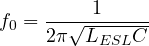
above which the capacitor behaves like an inductor and its impedance grows with frequency (Circuit Theory lesson on resonant circuits).
Example. 100 nF with 1 nH of inductance:  MHz. Above this frequency the inductance counts, not the capacitance: a larger capacitor does not help, one with shorter connections does. This is why small capacitors in tiny packages are placed right at the pins, with short vias to the planes; and for even higher frequencies the capacitance between closely spaced supply and ground planes, which has very low inductance, is exploited.
Layer stack-up
In multilayer boards the previous rules become stack-up choices. For a four-layer board the classic is: signals, ground, supply, signals. Each signal layer has an adjacent plane as reference, and closely spaced ground and supply form a distributed capacitor. The general rules:
- every signal layer adjacent to a plane, as close as possible;
- fast signals (clocks, high-speed lines) on inner layers between two planes, which shield them;
- supply plane slightly recessed relative to the ground plane (about 20 times the spacing between them), to reduce edge radiation;
- frequent ground vias along the edge, “stitching” the planes and closing slots.
Two-layer boards, which are cheap, can still be done well: one side almost entirely ground, short traces, and every fast signal with its return alongside.