Radiated emissions: differential-mode loops and common-mode cables
Differential-mode and common-mode emission formulas proved from elementary antennas, a numerical comparison with the limits, ferrites, filters and balanced signals.
Nobody designs a digital circuit to radiate, yet every circuit is an unintentional antenna. There are two mechanisms: loops carrying signal currents, which radiate in differential mode, and cables carrying small common-mode currents, which radiate like dipoles. The second, for the same current, is enormously more effective, and it is the cause of most test failures. In this lesson we derive the two emission formulas from the elementary antennas, compare them with a numerical example against legal limits, and see how each is reduced.
Differential mode and common mode
In a pair of conductors (a signal and its return) the current can always be split into two parts:
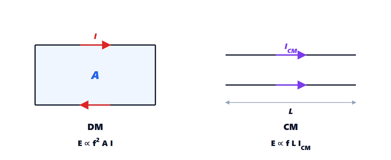
- differential mode (DM): equal and opposite currents in the two conductors,
 . It is the “intended” current, that of the signal;
- common mode (CM): equal currents in the same direction,
 , which return through parasitic capacitances to ground, the chassis or earth. Nobody wants it: it arises from asymmetries, from noise voltages on ground that push current along cables, from coupling.
Differential-mode emission
Theorem. A small loop of area  carrying current
 at frequency
 produces in the far field, at distance
 and in the direction of maximum emission, an electric field of amplitude

Proof. The far field of a small loop (magnetic dipole) is  , with
 Ω and
 (Antennas lesson on elementary dipoles). Substituting:

and  . In measurements there is also the reflecting ground plane of the test site, which can double the field. ∎
The field grows with the square of frequency: doubling the frequency of a harmonic quadruples the emission (+12 dB). It is reduced by shrinking the loop area, i.e. bringing the return close to the signal (lesson on the printed circuit board), and by reducing the current and its harmonic content (lesson on the spectrum).
Common-mode emission
Theorem. A cable of length  , short compared with the wavelength, carrying common-mode current , produces a maximum field

Proof. A short wire with uniform current is an elementary (Hertzian) dipole, with far field  (same lesson). The two conductors each carry
 in the same direction, so they are equivalent to a single wire with . Substituting and :

The doubled value in the formula accounts for reflection from the test site’s ground plane. ∎
The comparison
Example. At 100 MHz, at a distance of 3 m:
- a 1 cm² loop (
 m²) with 10 mA of signal current:
 µV/m, i.e. about 33 dBµV/m;
- a 1 m cable with 1 µA of common-mode current:
 µV/m, i.e. about 32 dBµV/m.
A common-mode current ten thousand times smaller than the signal current radiates just as much. The class B limit at 3 m in this band is about 40 dBµV/m: with 10 µA of common mode, a tiny amount, the cable reaches 52 dBµV/m and the test fails. The lesson is clear: cables are the main antennas, and emission problems are looked for on cables first. A radio-frequency current clamp around a cable measures directly and makes it possible to predict the test result on the bench.
Reducing common mode
The common-mode current on the cable is driven by a noise voltage between the circuit reference (the printed circuit board ground) and the “rest of the world”. The remedies:
- reduce the voltage that drives it: a continuous ground plane with low inductance, because the ground drop between the switching circuit and the point where the cable connects is precisely the source (lesson on the printed circuit board);
- a common-mode ferrite on the cable: it presents an impedance of a few hundred ohms to the common-mode current and almost none to the signal, because the fluxes of the outgoing and return conductors cancel (lesson on filters);
- filter every wire at the connector entry, with capacitors to the chassis;
- shield the cable, bonding the braid to the chassis at 360° (lesson on shielding);
- balanced differential signals: if the two halves are perfectly symmetrical, the conversion from differential to common mode is zero. Imbalance, even 1 %, converts part of the signal current into common-mode current: this is why differential pairs must be routed with identical lengths and spacings.