Production planning: MRP and sequencing rules

A factory must decide every day what to produce, in what quantities and in what order on the machines. Production planning translates orders and forecasts into plans, and scheduling establishes the sequence of jobs. In this lesson we look at hierarchical planning and MRP logic, sequencing rules on one machine with the proofs of the optimality of SPT and EDD, and Johnson’s rule for two machines with an example whose optimality is proved.

From planning to sequencing

Planning proceeds by levels, with shorter and shorter horizons:

1. the aggregate plan (months): capacity, shifts, inventory levels by product family;
2. the master production schedule (MPS, weeks): which finished products, how many and when;
3. material requirements planning (MRP): starting from the MPS and the bill of materials (the list of components of each product, level by level), the net quantities to produce or buy are computed for each component, subtracting available stock, together with the order release dates, brought forward by the lead time;
4. scheduling (days, hours): the sequence of jobs on each resource.

A car has thousands of components; an electronic board hundreds. Computing requirements by hand would be impossible: MRP was one of the first great applications of computers in business, and it is the heart of ERP systems.

One machine: SPT and EDD

jobs must be processed on one machine, with durations and due dates . Different rules optimise different objectives.

Theorem (SPT). Processing jobs in order of increasing duration (shortest processing time) minimises the mean completion time.

Proof. It is the same exchange argument as CPU scheduling (Operating Systems lesson on scheduling): if two consecutive jobs are in “long before short” order, swapping them brings the short one’s completion forward by the long one’s duration and delays the long one by the short one’s duration, so the sum decreases; the other jobs do not change. The optimum has no inversions. ∎

Theorem (EDD). Processing jobs in order of increasing due date (earliest due date) minimises the maximum lateness .

Proof. Consider two consecutive jobs and with and before , starting at time and both finishing by . Before the swap finishes at , with lateness , the larger of the two (because finishes before and has a later due date). After the swap finishes before , and finishes at with lateness . The maximum of the two does not increase, and the other jobs do not change. Removing the inversions one by one leads to the EDD order without getting worse. ∎

Neither rule is good for everything: SPT may make long jobs wait for a long time; EDD ignores durations. To minimise the number of late jobs there is a dedicated algorithm (Moore-Hodgson); for more complex objectives the problems quickly become intractable and heuristics are used.

Two machines: Johnson’s rule

Each job goes first on machine (duration ) and then on (duration ), in the same order. The goal is to minimise the total time (makespan). Johnson (1954) gave the optimal rule:

1. jobs with go first, in order of increasing ;
2. the others go last, in order of decreasing .

The idea is to keep busy as soon as possible (short jobs on at the start) and not to leave it with a lot of work at the end (short jobs on at the end).

Example. Five jobs : J1 (3, 6), J2 (5, 2), J3 (1, 2), J4 (6, 6), J5 (7, 5). First group, by increasing : J3, J1, J4. Second group, by decreasing : J5, J2. Sequence J3, J1, J4, J5, J2.

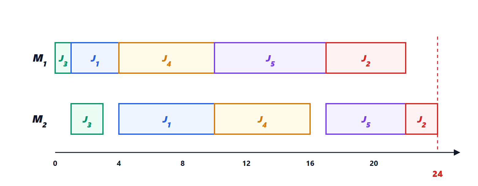
On the jobs finish at times 1, 4, 10, 17, 22; on at 3, 10, 16, 22, 24. The makespan is 24.

Optimality in the example. Any sequence must occupy for , and after the last job on at least its duration on is still needed, which is at least . So no sequence finishes before 24, and Johnson’s sequence reaches the bound. (The general proof again uses an exchange between adjacent jobs.)

With three or more machines the problem becomes NP-hard and heuristics are used; Johnson’s rule remains useful when two machines dominate, for example an assembly station followed by testing.