The coaxial cable from Maxwell's equations: characteristic impedance and why 75 Ω and 50 Ω

The TEM mode derived from Maxwell's equations, the coax field from Laplace's equation, Z0 = 60/√εr ln(b/a), proof of the minimum-loss (76.7 Ω), maximum-power (30 Ω) and maximum-voltage (60 Ω) ratios, the 50 Ω compromise, a TV cable number by number, Python code.

ielettronica 25 October 2026 11 min read 0 comments

Why are TV antenna cables 75 Ω and those of radios, instruments and Wi-Fi 50 Ω? It is not an arbitrary convention, nor a property of copper: it is the result of an optimisation that starts from Maxwell’s equations. This in-depth study derives the characteristic impedance of the coaxial cable directly from Maxwell’s equations, proves that it depends only on the ratio of the conductor diameters and on the dielectric, and then proves which ratio gives minimum loss (about 77 Ω, hence 75 Ω), which gives maximum power handling (30 Ω) and which maximum voltage (60 Ω). 50 Ω turns out to be a compromise. Python code checks all the numbers.

Impedance, not resistance

An ideal coaxial cable dissipates nothing, yet a generator connected to a very long cable (or one terminated in the right load) sees at its terminals a resistance of 75 Ω: it absorbs power like a resistor. The power is not turned into heat, but travels along the cable as a wave. The ratio between voltage and current of this wave is the characteristic impedance $Z_0$ . If the cable is terminated in a load equal to $Z_0$ the wave is absorbed without reflections; otherwise part of it comes back (transmission lines lesson). This is why antenna, cable and receiver must have the same $Z_0$ .

The TEM mode from Maxwell’s equations

In the dielectric between the conductors (permittivity $\varepsilon$ , permeability $\mu$ , no charges or currents) Maxwell’s equations for sinusoidal fields of angular frequency $\omega$ are

$\nabla\times\mathbf E = -j\omega\mu\mathbf H,\qquad \nabla\times\mathbf H = j\omega\varepsilon\mathbf E,\qquad \nabla\cdot\mathbf E = 0,\qquad \nabla\cdot\mathbf H = 0$

We look for a wave travelling along the cable axis $z$ , with fields $\mathbf E = \mathbf e(x, y)\,e^{-j\beta z}$ , $\mathbf H = \mathbf h(x, y)\,e^{-j\beta z}$ , all transverse (no component along $z$ ): the TEM (transverse electromagnetic) mode.

Theorem. For the TEM mode:

1. the transverse electric field is the gradient of a potential that satisfies Laplace’s equation in the cross-section: $\mathbf e = -\nabla_t\Phi$ , $\nabla_t^2\Phi = 0$ ;

2. the propagation constant is $\beta = \omega\sqrt{\mu\varepsilon}$ , so the velocity is $v = 1/\sqrt{\mu\varepsilon} = c/\sqrt{\varepsilon_r}$ (with $\mu = \mu_0$ );

3. the magnetic field is $\mathbf h = \frac{1}{\eta}\,\hat z\times\mathbf e$ , with $\eta = \sqrt{\mu/\varepsilon}$ : at every point $|\mathbf H| = |\mathbf E|/\eta$ .

Proof. 1. The $z$ component of Faraday’s law contains only transverse derivatives of the transverse fields: $(\nabla_t\times\mathbf e)_z = -j\omega\mu h_z = 0$ . A curl-free field is a gradient, $\mathbf e = -\nabla_t\Phi$ . Gauss’s law, with $e_z = 0$ , gives $\nabla_t\cdot\mathbf e = 0$ , i.e. $\nabla_t^2\Phi = 0$ .

2. and 3. The transverse components of Faraday’s law, with $\partial/\partial z = -j\beta$ and $e_z = 0$ , give $-j\beta\,\hat z\times\mathbf e = -j\omega\mu\mathbf h$ , i.e. $\mathbf h = \frac{\beta}{\omega\mu}\hat z\times\mathbf e$ . Likewise Ampère’s law gives 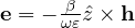$\mathbf e = -\frac{\beta}{\omega\varepsilon}\hat z\times\mathbf h$ . Substituting the first into the second and using $\hat z\times(\hat z\times\mathbf e) = -\mathbf e$ (since $\mathbf e$ is transverse): $\mathbf e = \frac{\beta^2}{\omega^2\mu\varepsilon}\mathbf e$ , so $\beta^2 = \omega^2\mu\varepsilon$ . Then $\frac{\beta}{\omega\mu} = \sqrt{\frac{\varepsilon}{\mu}} = \frac{1}{\eta}$ . ∎

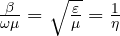Point 1 is the heart of the result: in the cross-section the electric field is identical to the electrostatic one between the two conductors. The TEM mode exists only if there are at least two separate conductors (in a waveguide, with a single conductor, $\Phi$ would be constant and the field zero): the coax has them, and propagates it at any frequency, even DC.

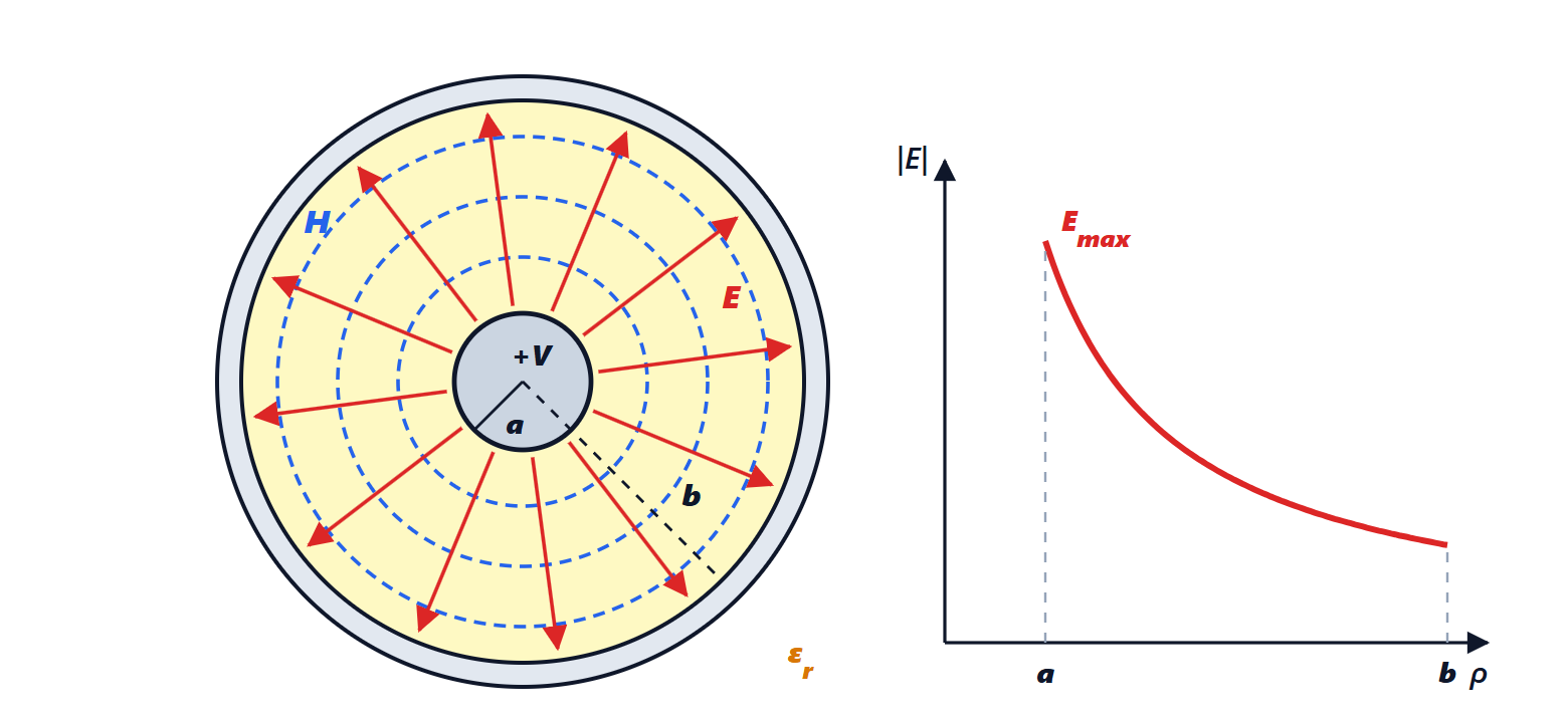
The field in the coax

The inner conductor has radius $a$ and potential $V$ , the outer one inner radius $b$ and potential 0. By symmetry $\Phi$ depends only on the distance $\rho$ from the axis, and Laplace’s equation in cylindrical coordinates becomes

$\frac{1}{\rho}\frac{d}{d\rho}\left(\rho\frac{d\Phi}{d\rho}\right) = 0 \;\Rightarrow\; \rho\frac{d\Phi}{d\rho} = \text{const} \;\Rightarrow\; \Phi = A\ln\rho + B$

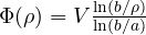With $\Phi(a) = V$ and $\Phi(b) = 0$ : $\Phi(\rho) = V\frac{\ln(b/\rho)}{\ln(b/a)}$ , so the field is radial and equals

$E_\rho = -\frac{d\Phi}{d\rho} = \frac{V}{\rho\ln(b/a)},\qquad H_\varphi = \frac{E_\rho}{\eta} = \frac{V}{\eta\,\rho\ln(b/a)}$

The magnetic field circles the axis. The current on the inner conductor follows from Ampère’s law on a circle of radius $\rho$ : $I = \oint H_\varphi\,dl = 2\pi\rho H_\varphi = \frac{2\pi V}{\eta\ln(b/a)}$ , independent of $\rho$ as it must be.

The TEM mode field in the coax cross-section — On the left the electric field lines, red, run radially from the inner to the outer conductor; the magnetic field lines, dashed blue, are circles around the axis. On the right the electric field strength decreases as 1 over rho: it is maximum on the surface of the inner conductor.

The characteristic impedance

The ratio between voltage and current of the wave is therefore

$Z_0 = \frac{V}{I} = \frac{\eta}{2\pi}\ln\frac{b}{a} = \frac{60\ \Omega}{\sqrt{\varepsilon_r}}\ln\frac{b}{a}$

(with $\eta = \eta_0/\sqrt{\varepsilon_r}$ and $\eta_0 = 376.7$ Ω $\approx 120\pi$ Ω, the impedance of free space: $\frac{\eta_0}{2\pi} = 59.96$ Ω). Here is the result: $Z_0$ depends neither on frequency nor on absolute size, but only on the ratio $b/a$ and on the dielectric. A cable as thick as a finger and one as thin as a hair have the same impedance if they have the same ratio.

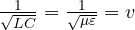Two checks. *With inductance and capacitance.* From Gauss’s law the capacitance per metre is $C = \frac{2\pi\varepsilon}{\ln(b/a)}$ ; from the magnetic flux between the conductors the inductance per metre is $L = \frac{\mu}{2\pi}\ln\frac{b}{a}$ . Then $\sqrt{L/C} = \frac{1}{2\pi}\sqrt{\mu/\varepsilon}\,\ln\frac{b}{a} = Z_0$ and $\frac{1}{\sqrt{LC}} = \frac{1}{\sqrt{\mu\varepsilon}} = v$ , as in the telegrapher’s equations. *With power.* The Poynting vector $\frac{1}{2}E_\rho H_\varphi$ , integrated over the annulus between $a$ and $b$ , gives $\int_a^b\frac{V^2}{2\eta\rho^2\ln^2(b/a)}2\pi\rho\,d\rho = \frac{V^2}{2}\cdot\frac{2\pi}{\eta\ln(b/a)} = \frac{V^2}{2Z_0} = \frac{1}{2}VI$ : power travels in the dielectric, not in the copper.

Why 75 Ω: minimum loss

A real cable attenuates the signal mainly through conductor resistance (the dielectric matters less, as long as it is good). At radio frequencies current flows in a surface layer a few micrometres thick (skin effect), with surface resistance $R_s = \sqrt{\pi f\mu_0/\sigma}$ .

Lemma. The resistance per metre of the coax is $R = \frac{R_s}{2\pi}\left(\frac{1}{a} + \frac{1}{b}\right)$ and the attenuation due to the conductors is $\alpha = \frac{R}{2Z_0}$ nepers per metre.

Proof. The current $I$ of the inner conductor spreads over the circumference $2\pi a$ : surface density $J_s = \frac{I}{2\pi a}$ . The power dissipated per metre is $\frac{1}{2}R_s|J_s|^2\cdot 2\pi a = \frac{1}{2}\frac{R_s}{2\pi a}I^2$ , i.e. a resistance $\frac{R_s}{2\pi a}$ ; the same for the outer conductor with $b$ . The transported power is $P = \frac{1}{2}Z_0I^2$ and it loses $\frac{1}{2}RI^2$ per metre, so $\frac{dP}{dz} = -\frac{R}{Z_0}P = -2\alpha P$ . ∎

The outer diameter of the cable is fixed by size, weight, cost and by the maximum frequency of use (see below). With $b$ fixed and $x = b/a$ :

$\alpha = \frac{R_s}{2\pi}\cdot\frac{1/a + 1/b}{2\cdot\frac{\eta}{2\pi}\ln x} = \frac{R_s}{2\eta b}\cdot\frac{1 + x}{\ln x}$

If the inner conductor is too thin (large $x$ ) its resistance grows; if it is too thick ( $x$ close to 1) the impedance becomes small and a lot of current is needed for the same power. There is an optimum.

Theorem (minimum loss). With the outer diameter fixed, the conductor attenuation is minimum for $x = b/a = 3.591$ , i.e. for $Z_0 = 76.7$ Ω in air.

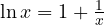Proof. $\frac{d}{dx}\frac{1 + x}{\ln x} = \frac{\ln x - \frac{1 + x}{x}}{\ln^2 x} = 0$ when $\ln x = 1 + \frac{1}{x}$ . The equation has no elementary solution; numerically $x = 3.5911$ (to the left the derivative is negative, to the right positive: it is a minimum). Then $Z_0 = 59.96\cdot\ln 3.5911 = 76.65$ Ω. ∎

The minimum is very flat: with 75 Ω in air the attenuation is only 0.03 % above the minimum, with 70 or 85 Ω a few tenths of a percent. This is why the nearby round number, 75 Ω, was chosen for all uses where losses matter and power does not: television and satellite reception, cable distribution, professional video. There is also a convenience: the half-wave dipole has 73 Ω.

An honest clarification: the optimum is in the ratio $b/a$ , not in the impedance. With a dielectric the optimum impedance becomes $76.7/\sqrt{\varepsilon_r}$ Ω: with solid polyethylene ( $\varepsilon_r = 2.25$ ) it is 51 Ω. Modern TV cables use foamed polyethylene ( $\varepsilon_r \approx 1.5$ ) and to reach 75 Ω have $b/a = 4.63$ : conductor attenuation is 2.3 % above the minimum, a negligible difference compared with the advantage of a single standard.

Maximum power and maximum voltage

The power a cable can carry is limited by breakdown in the dielectric: the field must not exceed a value $E_{max}$ (about 3 MV/m in dry air). The field is maximum on the inner conductor, $E(a) = \frac{V}{a\ln x}$ .

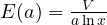Theorem (maximum power). With $b$ and $E_{max}$ fixed, the power that can be carried is maximum for $x = \sqrt e = 1.649$ , i.e. $Z_0 = 30.0$ Ω in air.

Proof. The maximum voltage is $V = E_{max}\,a\ln x = E_{max}\,b\,\frac{\ln x}{x}$ . The power is $P = \frac{V^2}{2Z_0} = \frac{E_{max}^2b^2\ln^2x/x^2}{2\frac{\eta}{2\pi}\ln x} = \frac{\pi E_{max}^2b^2}{\eta}\cdot\frac{\ln x}{x^2}$ . The derivative of $\frac{\ln x}{x^2}$ is $\frac{1 - 2\ln x}{x^3}$ , zero for $\ln x = \frac{1}{2}$ . Then $Z_0 = 59.96\cdot\frac{1}{2} = 30.0$ Ω. ∎

Theorem (maximum voltage). With $b$ and $E_{max}$ fixed, the voltage that can be withstood is maximum for $x = e$ , i.e. $Z_0 = 60.0$ Ω in air.

Proof. $V \propto \frac{\ln x}{x}$ , with derivative $\frac{1 - \ln x}{x^2}$ , zero for $\ln x = 1$ . ∎

The three quantities as a function of impedance, in air, with fixed outer diameter — Maximum power, orange, peaks at 30 ohms; maximum voltage, green, at 60 ohms; the inverse of attenuation, blue, at 76.7 ohms. Each curve is divided by its own maximum. The dashed red lines mark 50 and 75 ohms.

And 50 Ω?

No impedance is optimal for everything: 30 Ω for power, 77 Ω for losses. Those who transmit (radio, radar, base stations, laboratory instruments that must suit everything) want both. 50 Ω is the compromise: it is close to both the arithmetic mean (53 Ω) and the geometric mean (48 Ω) of the two optima. In air, at 50 Ω attenuation is 10 % above the optimum and 86 % of the maximum power is carried; at 75 Ω attenuation is minimum but power drops to 56 %. There is also a coincidence often quoted: a cable with the minimum-loss ratio and solid polyethylene dielectric has exactly 51 Ω.

	$b/a$	$Z_0$ in air	$Z_0$ with $\varepsilon_r = 2.25$	use
minimum loss	3.591	76.7 Ω	51.1 Ω	TV, satellite, video (75 Ω)
maximum voltage	2.718	60.0 Ω	40.0 Ω	high-voltage pulses
maximum power	1.649	30.0 Ω	20.0 Ω
compromise	2.302	50 Ω	33.3 Ω	radio, instruments, Wi-Fi (50 Ω)

A TV cable, number by number

Foamed polyethylene dielectric ( $\varepsilon_r = 1.5$ ) with 4.6 mm diameter, impedance 75 Ω (roughly the dimensions of an RG-6):

ratio $b/a = e^{75\sqrt{1.5}/59.96} = 4.63$ , hence an inner conductor of 0.99 mm;
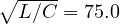$C = 54.5$ pF/m, $L = 306$ nH/m, $\sqrt{L/C} = 75.0$ Ω;
velocity $v = c/\sqrt{1.5} = 0.816\,c$ (the “velocity factor” printed in catalogues);
attenuation of the copper conductors alone at 1 GHz: $R_s = 8.2$ mΩ, $R = 3.2$ Ω/m, $\alpha = R/(2Z_0) = 0.021$ Np/m, i.e. 18.6 dB per 100 m, the typical catalogue value (dielectric losses add little);
the TEM mode is not the only possible one: above the cutoff frequency of the first higher mode, TE₁₁, with cutoff wavelength about $\pi(a + b)$ , the cable would also carry that, with distortion. Here $f_c = \frac{c}{\pi(a + b)\sqrt{\varepsilon_r}} \approx 28$ GHz: this is why cables for millimetre waves must be thin, and the outer diameter cannot be increased at will to reduce losses.

The calculation in Python

import numpy as np
from scipy.optimize import brentq, minimize_scalar

eta0 = 119.9169832 * np.pi                 # impedance of free space, 376.73 ohm
Z0 = lambda x, er=1.0: eta0 / (2 * np.pi * np.sqrt(er)) * np.log(x)    # x = b/a

# 1) minimum attenuation with fixed outer diameter: minimum of (1 + x)/ln x
x_att = brentq(lambda x: x * np.log(x) - 1 - x, 2, 6)
# 2) maximum power with fixed maximum field: maximum of ln x / x^2
x_pow = np.sqrt(np.e)
# 3) maximum voltage with fixed maximum field: maximum of ln x / x
x_v = np.e
for name, x in (("minimum loss", x_att), ("maximum power", x_pow), ("maximum voltage", x_v)):
    print(f"{name:17s}: b/a = {x:.4f}, Z0 air = {Z0(x):.2f} ohm, Z0 polyethylene (er 2.25) = {Z0(x, 2.25):.2f} ohm")
# numerical check of the optima
print("check:", round(minimize_scalar(lambda x: (1 + x) / np.log(x), bounds=(1.1, 10), method="bounded").x, 4),
      round(minimize_scalar(lambda x: -np.log(x) / x**2, bounds=(1.01, 10), method="bounded").x, 4))
print("means of 30 and 76.7: arithmetic", round((Z0(x_pow) + Z0(x_att)) / 2, 1), "geometric", round(np.sqrt(Z0(x_pow) * Z0(x_att)), 1))
# cost of choosing 50 ohm instead of the optimum (in air)
att = lambda x: (1 + x) / np.log(x)
pw = lambda x: np.log(x) / x**2
x50 = np.exp(50 * 2 * np.pi / eta0)
x75 = np.exp(75 * 2 * np.pi / eta0)
print(f"50 ohm air: b/a = {x50:.3f}, attenuation +{100 * (att(x50) / att(x_att) - 1):.1f} %, power {100 * pw(x50) / pw(x_pow):.1f} % of maximum")
print(f"75 ohm air: b/a = {x75:.3f}, attenuation +{100 * (att(x75) / att(x_att) - 1):.2f} %, power {100 * pw(x75) / pw(x_pow):.1f} % of maximum")
# TV cable with foamed dielectric er = 1.5 and 4.6 mm dielectric diameter: inner conductor for 75 ohm
er, D = 1.5, 4.6e-3
x = np.exp(75 * 2 * np.pi * np.sqrt(er) / eta0)
d = D / x
print(f"TV cable: b/a = {x:.3f}, inner d = {d * 1e3:.2f} mm, v = {1 / np.sqrt(er):.3f} c")
# L and C per metre and check Z0 = sqrt(L/C)
mu0, e0 = 4e-7 * np.pi, 8.8541878128e-12
C = 2 * np.pi * e0 * er / np.log(x)
L = mu0 / (2 * np.pi) * np.log(x)
print(f"C = {C * 1e12:.1f} pF/m, L = {L * 1e9:.0f} nH/m, sqrt(L/C) = {np.sqrt(L / C):.2f} ohm")
# cutoff frequency of the first higher mode TE11 (approximation lambda_c = pi (a + b))
a, b = d / 2, D / 2
fc = 299792458 / (np.pi * (a + b) * np.sqrt(er))
print(f"TE11: fc = {fc / 1e9:.1f} GHz")
# conductor attenuation at 1 GHz (copper), alpha = R / (2 Z0), R = Rs/(2 pi) (1/a + 1/b)
f, sigma = 1e9, 5.8e7
Rs = np.sqrt(np.pi * f * mu0 / sigma)
R = Rs / (2 * np.pi) * (1 / a + 1 / b)
alpha = R / (2 * 75)
print(f"1 GHz: R = {R:.3f} ohm/m, alpha = {alpha:.4f} Np/m = {8.686 * alpha * 100:.1f} dB/100 m")

Running it prints the three optima (3.5911 and 76.65 Ω, 1.6487 and 29.98 Ω, 2.7183 and 59.96 Ω), the means 53.3 and 47.9 Ω, the costs of choosing 50 Ω (+10.3 % attenuation, 85.5 % of the power) and 75 Ω (+0.03 %, 55.7 %), and the TV cable numbers: 0.99 mm, 54.5 pF/m, 306 nH/m, 75.00 Ω, 27.9 GHz and 18.6 dB/100 m.

0 Comments

Oldest

Newest Most Voted

Cookie	Duration	Description
cookielawinfo-checkbox-analytics	11 months	This cookie is set by GDPR Cookie Consent plugin. The cookie is used to store the user consent for the cookies in the category "Analytics".
cookielawinfo-checkbox-functional	11 months	The cookie is set by GDPR cookie consent to record the user consent for the cookies in the category "Functional".
cookielawinfo-checkbox-necessary	11 months	This cookie is set by GDPR Cookie Consent plugin. The cookies is used to store the user consent for the cookies in the category "Necessary".
cookielawinfo-checkbox-others	11 months	This cookie is set by GDPR Cookie Consent plugin. The cookie is used to store the user consent for the cookies in the category "Other.
cookielawinfo-checkbox-performance	11 months	This cookie is set by GDPR Cookie Consent plugin. The cookie is used to store the user consent for the cookies in the category "Performance".
viewed_cookie_policy	11 months	The cookie is set by the GDPR Cookie Consent plugin and is used to store whether or not user has consented to the use of cookies. It does not store any personal data.

Impedance, not resistance

The TEM mode from Maxwell’s equations

The field in the coax

The characteristic impedance

Why 75 Ω: minimum loss

Maximum power and maximum voltage

And 50 Ω?

A TV cable, number by number

The calculation in Python

Related articles

how to install TP-Link wifi dongle drivers to raspberry PI (realtek driver)

The chips and sensors behind China’s assisted driving

Antenna temperature, G/T and antenna measurements

Deep dive: designing an airport surveillance radar step by step, from requirements to power

From imitation to reinforcement learning: how Chinese driving systems are trained

Remove the MacBook screen so it can work as a desktop computer