Impedance matching, the quarter-wave transformer and the Smith chart
Load reflection coefficient, input impedance with proof, notable cases, measures of mismatch, the quarter-wave transformer, the Smith chart and stubs.
A line terminated in a load different from its characteristic impedance reflects part of the power: the load receives less, the line fills with standing waves and the transmitter can be damaged. Moreover, the impedance seen at the input of the line changes with its length, sometimes in surprising ways. In this lesson we derive the input impedance of a line, the notable cases, the quarter-wave transformer and the graphical tool that sums them all up: the Smith chart.
The load reflection coefficient
A lossless line of impedance  is terminated at
 in a load
 . There,
 must hold, and with the solutions from the previous lesson:

If  there is no reflected wave: the line is matched. With a short-circuit load
 , with an open circuit
 .
Input impedance
Theorem. The impedance seen at distance  from the load is
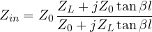
Proof. At distance from the load (that is at  ):

Substituting  , multiplying numerator and denominator by
 and using
 :

and dividing by  gives the formula. ∎
Notable cases
- Matched line ():
 at any length.
- Short circuit:
 , purely reactive. A short section (less than
 ) behaves as an inductor, between and
 as a capacitor. At radio frequencies inductors and capacitors are built this way from a piece of trace.
- Open circuit:
 , the opposite behaviour.
- Half-wave line (
 ,
 ):
 , the line is “transparent”.
- Quarter-wave line (
 ,
 ):

The quarter wave inverts the impedance: a short circuit becomes an open circuit and vice versa.
Measures of mismatch
A mismatched load is described by several equivalent quantities, all obtainable from  :
- the VSWR,
 (lesson on reflection);
- the return loss,
 dB: how much weaker the reflected wave is;
- the mismatch loss,
 dB: how much less power reaches the load.
Example. A 100 Ω load on a 50 Ω line:  , VSWR = 2, return loss 9.5 dB, and 89% of the power reaches the load (a 0.51 dB loss).
The quarter-wave transformer
To match the 100 Ω load to the 50 Ω line, a section of line with impedance  is inserted. At the input of the section one sees
 , which must equal 50 Ω:

The limit is bandwidth: the length is exactly only at one frequency, and away from it the match degrades. Cascading several sections with graded impedances widens the bandwidth.
The Smith chart
All these formulas can be “seen” on a single chart. The idea is to plot the reflection coefficient  in the complex plane: all passive loads lie inside the circle
 . On this circle the grid of the normalised impedance
 is drawn, related to by the transformation

which maps lines of constant real part into circles and lines of constant imaginary part into circular arcs.
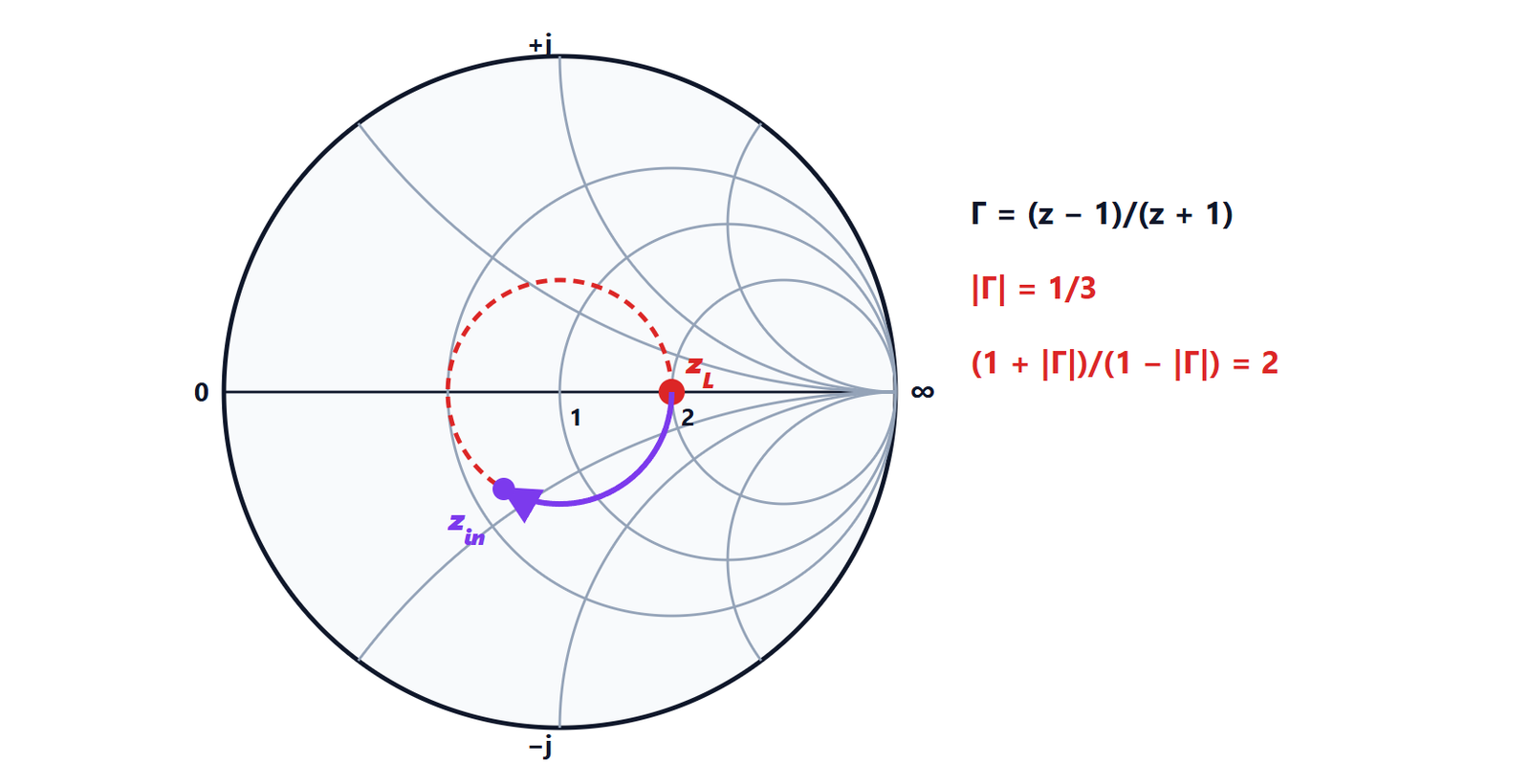
Moving along a lossless line multiplies by  : the magnitude stays the same and the phase rotates. On the chart the point turns around the centre on a constant-VSWR circle, clockwise when moving towards the generator, and makes a full turn every . The input impedance can then be read directly on the grid.
Single-stub matching. The classic method to match any load: move along the line until the real part of the normalised admittance equals 1 (you meet the  circle on the admittance chart), then add in parallel a stub, a short-circuited section of line whose length is chosen to cancel the imaginary part. Today the same calculations are done with a program or directly on the network analyser, which displays its measurements on a Smith chart; but the chart is still the most immediate way to understand what is going on.