Impedance matching with L-networks
Maximum transfer with conjugate matching proved, L-network formulas proved with a 100 MHz example, quality factor and bandwidth, multi-section networks, tunable networks.
A 20 Ω antenna, the input of a transistor of 10 Ω with a capacitive part, a filter designed for 50 Ω: to transfer maximum power and avoid reflections, one impedance must be transformed into the other with a lossless network. With transmission lines quarter-wave sections and the Smith chart are used (Electromagnetic Fields lesson on matching); with lumped components the simplest solution is the L-network. In this lesson we look at the maximum power transfer theorem with complex loads, the design of the L-network with the proof of its formulas and a numerical example, the link between quality factor and bandwidth, and multi-element networks.
Maximum power transfer
Theorem. A source with internal impedance  delivers maximum power to a load
 , i.e.
 and
 (conjugate matching).
Proof. With RMS voltage  , the power in the load is
 . The reactance appears only in the denominator, added squared:
 is maximum for , which cancels that term. What remains is
 , maximum for (Circuit Theory lesson on maximum power transfer). ∎
A lossless matching network must therefore make the source see the conjugate of its own impedance; if source and load are resistive, it must transform one resistance into another.
The L-network
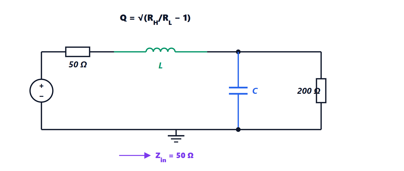
To match a low resistance  to a high one
 , a reactance is placed in series on the low-resistance side and a reactance in parallel on the high-resistance side, of opposite sign.
Theorem. With

and reactances of opposite sign, the network transforms into .
Proof. The parallel combination of and  is converted to its series equivalent. The admittance is
 ; with
 , the equivalent impedance is

(obtained by multiplying numerator and denominator by the conjugate). For the real part to be we need  , i.e. the first formula. The imaginary part then has magnitude
 , and the series reactance, of opposite sign and equal magnitude,
 , cancels it. What remains is
 . ∎
Example. Match 200 Ω to 50 Ω at 100 MHz:  .
 Ω, i.e.
 nH;
 Ω, i.e.
 pF. The version with the capacitor in series and the inductor in parallel works just as well: the first is a low-pass (it also attenuates harmonics, useful after a power amplifier), the second a high-pass (it lets DC bias through if it needs to be blocked elsewhere).
Quality factor and bandwidth
Matching is exact at a single frequency; moving away, the reactances change and the mismatch grows. The  of the L-network is fixed by the resistance ratio, and the bandwidth over which the match is good is roughly inversely proportional to (lesson on resonant circuits). Large ratios give large and narrow bandwidth: matching 1 Ω to 50 Ω requires
 .
- For wider bandwidth several L-sections are cascaded, each with a small ratio: with two sections one passes through the intermediate resistance
 (the geometric mean), and each section has a lower . It is the same principle as multi-section line transformers.
- For narrow bandwidth and a freely chosen (for instance to filter harmonics) π or T networks are used, seen as two L-networks back to back through a virtual resistance.
In practice components have losses (an inductor at 1 GHz may have an intrinsic of 30-50) and parasitics, and networks are optimised with a simulator starting from the analytical design. Above a few gigahertz lumped components give way to line sections on the printed circuit board (microstrip), with the same principles.
A typical case
A phone’s antenna changes impedance depending on how the phone is held: the nearby hand adds capacitance and losses. Modern phones use tunable matching networks, with digitally controlled variable capacitors, which software adjusts by measuring the reflected power. It is the matching of this lesson performed in real time, dozens of times a second.