Software radio: bandpass sampling and I/Q receivers
The bandpass sampling condition proved with an example, the jitter limit proved, the direct-conversion receiver, image rejection with I/Q imbalance proved.
In modern radios the analogue part has shrunk to a minimum: an amplifier, a mixer or not even that, and then an analogue-to-digital converter; filtering, demodulation and decoding are software. This is software-defined radio (SDR), from the phone to the base station. The heart of the problem moves to sampling and to the accuracy of the in-phase and quadrature branches. In this lesson we look at bandpass sampling with the proof of the non-overlap condition and an example, the limit due to sampling-time uncertainty, the direct-conversion receiver, and the image rejection ratio with its proof and an example.
Bandpass sampling
The sampling theorem (Signal Theory lesson on sampling) requires sampling at more than twice the maximum frequency. But a radio signal occupies only a narrow band  of width
 , far from zero: a sampling frequency related to
 suffices, provided the spectral replicas do not overlap. This is undersampling.
Theorem. A real signal with band can be sampled without overlap at frequency  if and only if, for some integer
 with
 ,
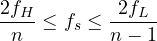
(for  the upper limit is absent and the ordinary condition
 is recovered).
Proof. The spectrum of a real signal occupies the positive band and its negative image  ; sampling replicates them at all multiples of . The replicas of the positive band are shifted by multiples of and do not overlap each other if
 . The risk is that a replica of the negative band,
 , falls on the positive band. The negative replicas all lie outside if one of them, the
 -th, lies entirely to the left, and the next, the -th, entirely to the right:
 and
 . These are the two inequalities of the statement. The interval is non-empty only if
 , i.e.
 . ∎
Example. A 70 MHz intermediate frequency with 10 MHz bandwidth, i.e. from 65 to 75 MHz. With  :
 MHz. A converter at 56 MHz correctly samples a 70 MHz signal, and the band reappears between 9 and 19 MHz, where it is processed digitally. With
 one could go down to about 21.5 MHz, but the allowed interval (from 21.43 to 21.67 MHz) is so narrow that clock tolerances make it impractical.
The converter must however have an analogue bandwidth reaching  , and a bandpass filter in front must remove everything outside , because every Nyquist zone folds onto the same digital band.
Sampling-time uncertainty
When sampling a high-frequency signal, a small error in the sampling instant (clock jitter) becomes a large amplitude error, because the signal changes rapidly.
Theorem. An RMS jitter  limits the signal-to-noise ratio of a sinusoid of frequency
 to

Proof. For  , a timing error
 produces an error
 . With independent of the signal, the mean square error is
 , that of the signal
 : the ratio is
 . ∎
Example. At 75 MHz with 1 ps of jitter:  dB, i.e. about 11 effective bits (lesson on quantisation), whatever the converter’s number of bits. Direct sampling at gigahertz frequencies needs clocks with jitter of tens of femtoseconds.
The direct-conversion receiver
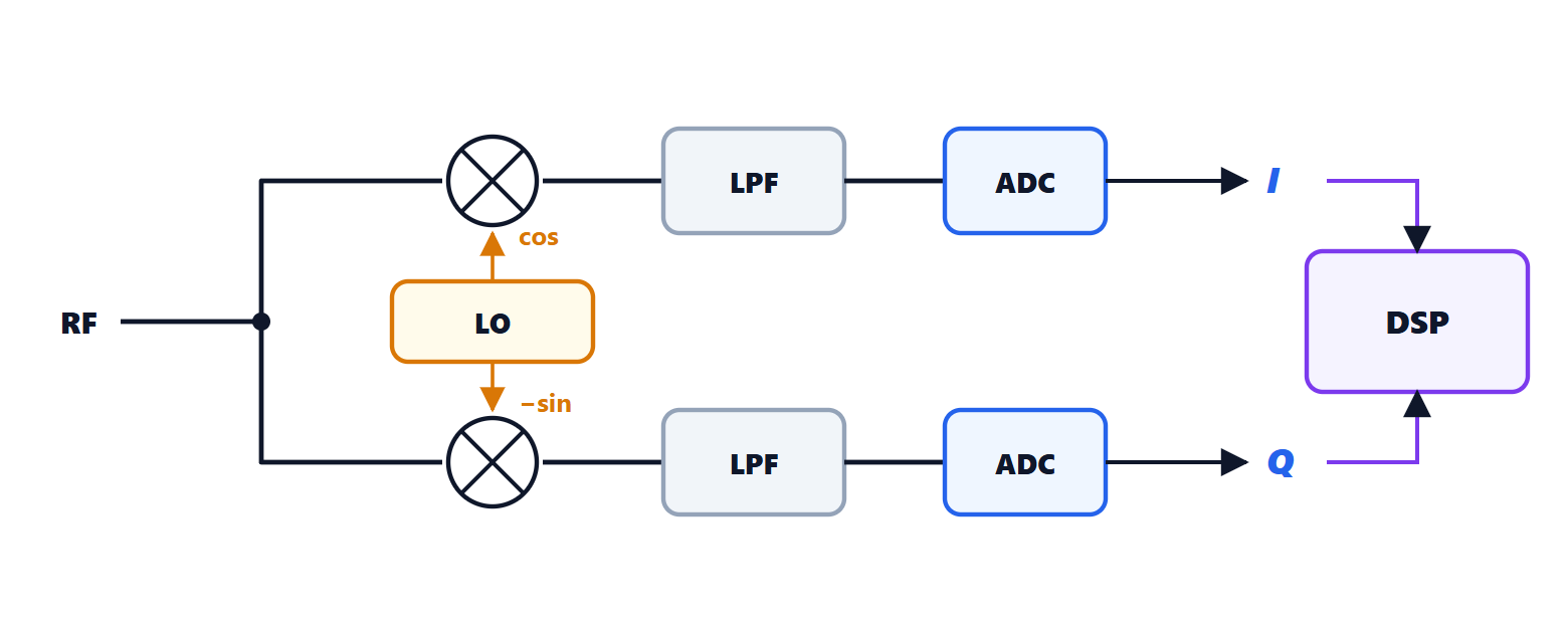
In the direct-conversion (or zero-IF) receiver the local oscillator is at the same frequency as the carrier, and the signal goes straight down to baseband. Two branches are needed, multiplied by cosine and sine: the two components I (in phase) and Q (quadrature) form the complex signal  , which distinguishes positive from negative frequencies, i.e. what lies above the carrier from what lies below it. A single branch would superimpose them. There is no image frequency to be filtered with external components, and channel filters become integrated low-pass filters: this is the architecture of almost all integrated transceivers. Its problems are the DC offset at the output (the local oscillator mixing with itself), flicker noise at baseband and imbalance between the branches.
I/Q imbalance
If the two branches are not perfectly equal, with a relative gain error  and a phase error
 relative to the ideal 90°, a signal at frequency
 leaves a residue at
 : the channel mirrored about the carrier interferes with the wanted one.
Theorem. The image rejection ratio is

Proof. The ideal complex oscillator is  . With the errors it becomes
 . Writing cosine and sine with complex exponentials, this is
 with
 and
 . The first term brings the wanted signal to baseband, the second the image. The power ratio is
 . For small errors the numerator is about 4, and the denominator
 . ∎
Example. Gain error of 1 % and phase error of 1° (0.0175 rad):  , about 40 dB. With analogue components one does not go much beyond 30-40 dB; modern receivers estimate and correct the imbalance digitally, reaching 60-70 dB. It is a typical example of modern radio: imperfect analogue electronics plus digital processing that compensates for its defects.