Taylor and Laurent series, singularities and poles
Radius of convergence and singularities, Laurent series in an annulus, removable, pole and essential singularities, isolated zeros and the identity principle, poles in systems.
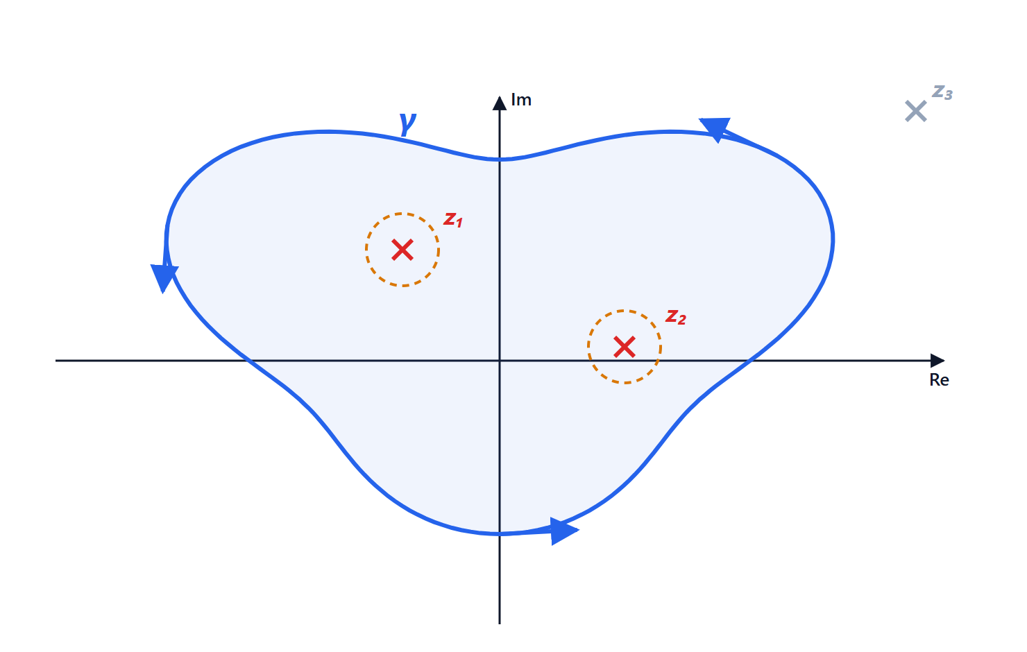
A holomorphic function can be expanded in a Taylor series around every point, and the series converges up to the nearest singularity. But what happens around a singularity? The answer is the Laurent series, which allows negative powers too. Singularities, which in a physical system are the poles of the transfer function, determine its entire behaviour.
Taylor series in the complex field
Theorem. If  is holomorphic in the disc
 , then throughout the disc

The proof starts from Cauchy’s integral formula and expands  as a geometric series. The consequence is remarkable: the radius of convergence is the distance to the nearest singularity.
This explains a mystery of real analysis. The function  is perfectly regular on the whole real line, yet its Taylor series at 0,
 , converges only for
 . The reason is visible only in the complex plane:
 has two singularities at
 , at distance 1 from the origin.
The Laurent series
Theorem. If is holomorphic in the annulus  , then

with coefficients  , computed round any circle in the annulus.
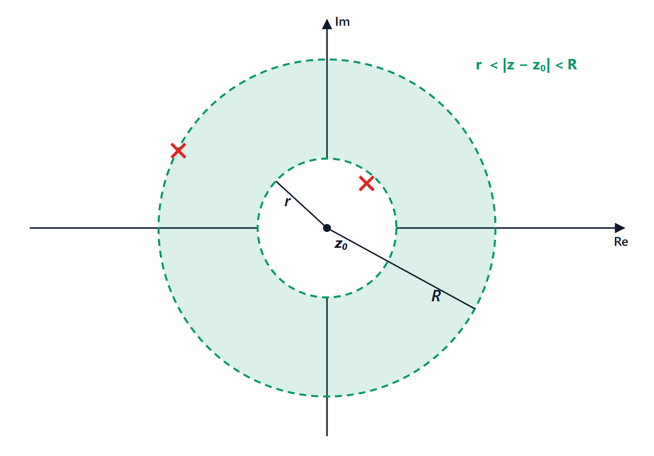
 converges in the green annulus between radii
 and
 : the inner circle passes through the nearest singularity, the outer one through the next.
The expansion depends on the annulus: the same function has different Laurent expansions in different annuli.
Example. 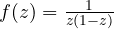 has singularities at 0 and 1. With partial fractions
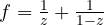 .
- For
 :
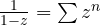 , so

- For
 :
 , so

In practice the coefficients are almost never computed with integrals: known series (geometric, exponential, sine, cosine) and their manipulations are used instead.
Classifying isolated singularities
A point where is not holomorphic, but is holomorphic in a punctured neighbourhood around it, is an isolated singularity. Its type depends on the principal part of the Laurent series in  .
| Type | Principal part | Behaviour | Example at  |
|---|---|---|---|
| removable | none | has a finite limit |  |
pole of order  | finite, up to  |  |  , double pole |
| essential | infinite | no limit |  |
Removable singularity.  : setting
 makes the function holomorphic. It is the standard limit of Analysis 1 seen from above.
Pole. has a pole of order at if and only if  has a finite non-zero limit. For rational functions
 the poles are the zeros of the denominator that do not cancel with the numerator, and the order is their multiplicity.
Essential singularity.  has infinitely many negative terms. Approaching 0 along the positive real axis it goes to
 , along the negative axis to 0, along the imaginary axis it oscillates with no limit. Picard’s theorem says that in every neighbourhood of an essential singularity the function takes every complex value, with at most one exception: wild behaviour, very different from poles.
Zeros and poles
If a holomorphic is not identically zero, its zeros are isolated: around each zero there is a neighbourhood with no other zeros. The identity principle follows: two holomorphic functions that agree on a segment, however small, agree everywhere. This is the “rigidity” of holomorphic functions: knowing how a linear circuit behaves at real frequencies determines its transfer function over the whole complex plane.
Why poles matter in engineering
The transfer function of a linear circuit or system is a rational function  . Its poles tell how the system behaves when left to itself: each pole
 produces a term
 in the response. Their position in the complex plane decides whether the system is stable, whether it oscillates and how quickly it settles, as we will see in the lessons on the Laplace transform. The zeros tell which frequencies the system blocks: a notch filter has zeros on the imaginary axis at the frequency to be removed.