Z transform in depth: stability, z plane, ZOH, Euler and Tustin
Properties and theorems proved, three inversion methods, stability with poles in the unit circle, the map z equals e to the sT, discretisation with hold, Euler and Tustin with prewarping, Python example, tables.
This page goes deeper into the lesson on the Z transform, the tool used to design every system that runs on a processor: digital filters, controllers in microcontrollers, car ECUs. It proves the properties and the initial and final value theorems, works out the inverse transform with three methods, proves the stability criterion (poles inside the unit circle), explains how the map  transforms the
 plane into the
 plane and compares the methods for going from a continuous system to a discrete one: zero-order hold, Euler and Tustin. At the end are the tables to remember and a Python example.
The properties, proved
Definition:  , for sequences that are zero for
 .
- Delay by
 samples.
 , with
 , becomes
 (terms with
 are zero).
- Advance.
 . More generally
 : initial conditions enter as in Laplace.
- Scaling.
^{-n} = X(z/a)](https://www.electronics-engineering.com/wp-content/ql-cache/quicklatex.com-874425c931e2063e8dfc6e6ac10b6135_l3.png "Rendered by QuickLaTeX.com") : multiplying by
 moves the poles by a factor
 .
- Multiplication by
 . Differentiating
 with respect to :
 , so
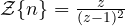
 . From
 one gets
 .
- Convolution.
 .
Theorem (initial and final values).  . If the poles of
 lie inside the unit circle,
 .
Proof. The first: as  all the terms
 with
 tend to 0. The second:
 . As
 the left-hand side tends to
 (telescoping series), so
 . ∎
The inverse transform: three methods
1. Partial fractions of  . Expand
 and multiply back by , so each term is
 . For a double pole,
 .
2. Long division. Divide the numerator by the denominator in powers of  : the coefficients of the quotient are the samples. It does not give a closed formula, but it is exactly what the processor does when it runs the difference equation.
3. Residues.  at the poles of
 : this is the inversion formula, an integral around a circle in the region of convergence (lessons on Cauchy’s formula and residues).
Stability, proved
A discrete system is stable (BIBO: bounded input, bounded output) if and only if its impulse response is summable,  .
Theorem. A system with rational  is stable if and only if all its poles have modulus less than 1.
Proof. With partial fractions,  is a combination of terms
 , one for each pole
 ( less than the multiplicity). If
 ,
 converges (ratio test: the ratio tends to ), and the sum of finitely many convergent series converges. If instead a pole has
 , the corresponding term does not tend to zero (for
 it has constant or growing modulus), so is not summable. Finally, if
 and
 ,
 : bounded output. ∎

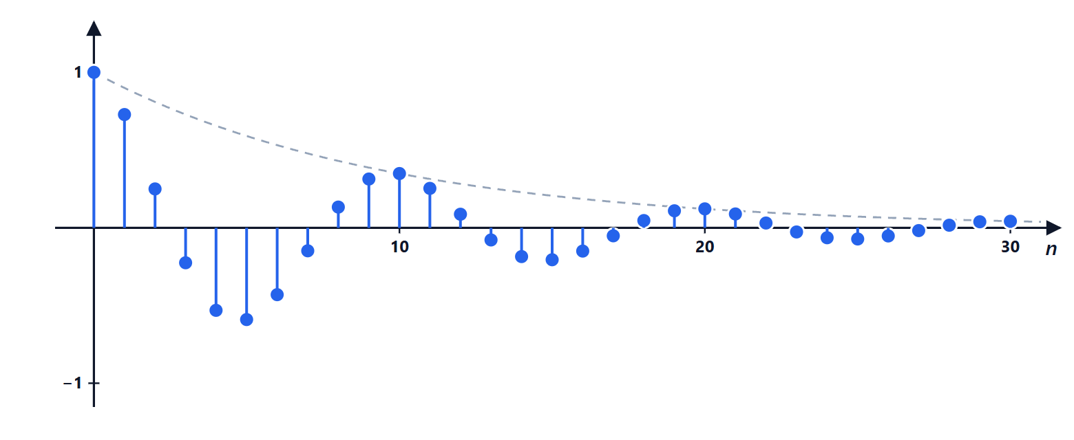
A negative pole has no continuous counterpart: it produces an oscillation at the Nyquist frequency (one sample up, one down). Complex poles  produce
 : damping given by the modulus, frequency by the angle.
In practice, to check stability without computing the poles one uses the Jury criterion (Digital Control lesson), or the bilinear transformation  , which maps the unit circle onto the left half of the
 plane, and then the Routh criterion.
From the s plane to the z plane
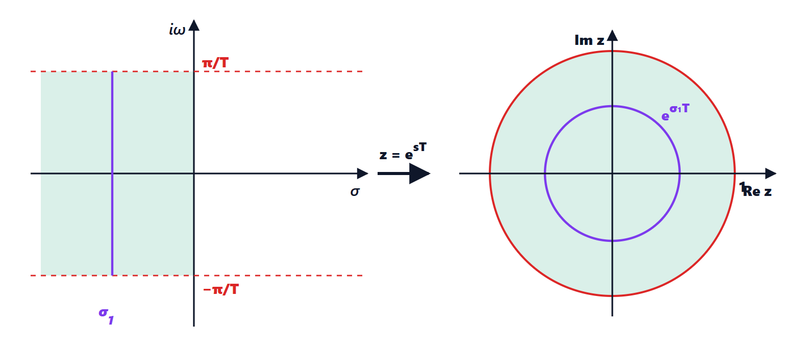
Sampling with period  , a continuous pole
 becomes the discrete pole
 (the sampled term
 is
 ). With
 :
 and
 .
- the left half-plane (
 ) goes inside the unit circle, the imaginary axis onto the circle;
- a vertical line
 goes into a circle of radius
 : constant settling time;
- the map is not one-to-one: and
 go to the same . The strip
 alone already covers the plane, and frequencies outside that strip are confused with those inside: this is aliasing, seen from the complex plane.
Discretising: ZOH, Euler, Tustin
A controller designed in continuous time,  , must be turned into a
 to run on the processor. The main methods:
Zero-order hold (ZOH). It is the exact model of a continuous process  driven by a D/A converter that holds its output constant between samples:

Proof. The discrete impulse, after the hold, is a pulse of duration :  . Its output is the step response
 minus the same delayed by . Sampled and transformed, it gives
 . ∎
For  :
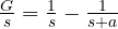 , so
 . The pole is exactly
 .
Forward Euler:  (derivative approximated with the forward difference). Backward Euler:
 . Tustin (bilinear transformation, trapezoidal rule):
 .
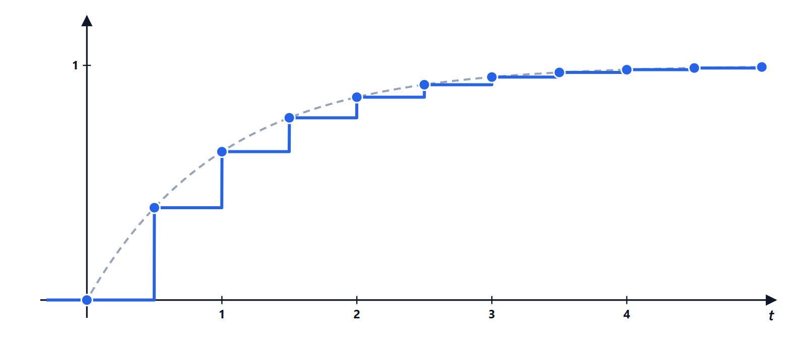
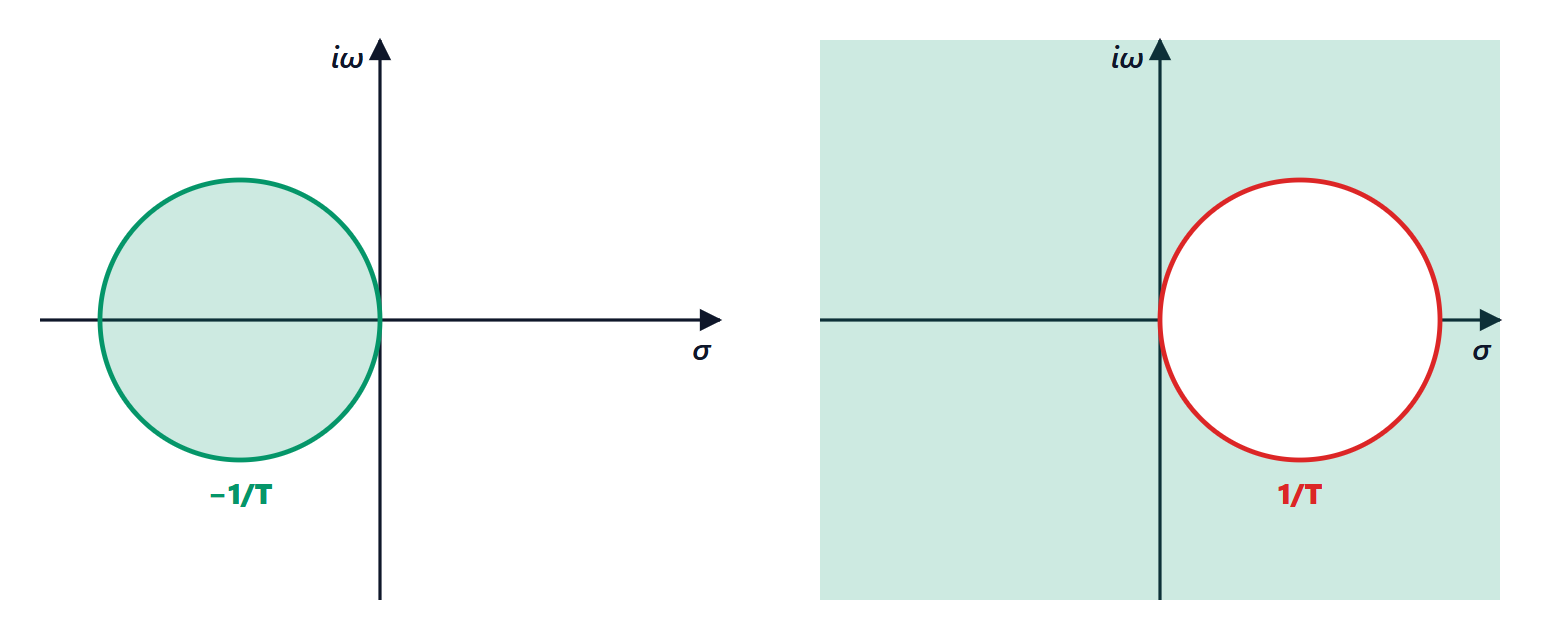
Theorem. Tustin maps the left half-plane exactly into the unit circle: a stable continuous controller stays stable for every . Forward Euler does not: a stable continuous pole becomes unstable if is too large.
Proof. Tustin:  . With
 , the numerator is closer to the origin than the denominator (they are symmetric about the imaginary axis, and
 lies on the left), so
 . Forward Euler:
 . The disc corresponds in to the disc
 : only poles inside that disc stay stable. A real pole
 becomes
 , unstable for
 . ∎
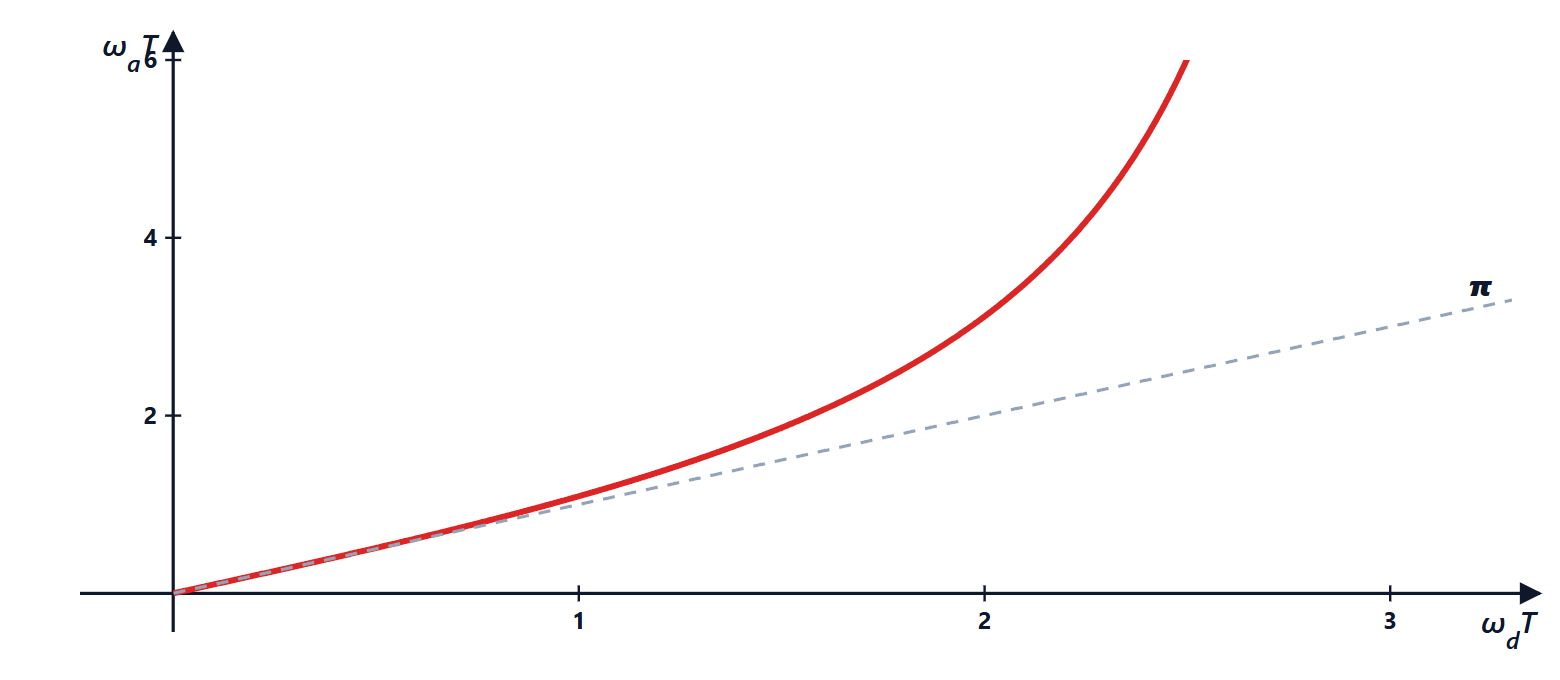
The price of Tustin: frequency warping. On the circle  , the substitution gives
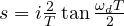 : the digital angular frequency
 corresponds to the analogue angular frequency
 . For small
 the two coincide; near Nyquist the tangent blows up. To make an important frequency coincide (for example the cut-off of a filter, or the crossover of a controller) one uses prewarping: the continuous design is done at the corrected frequency
 .
Frequency response of discrete systems
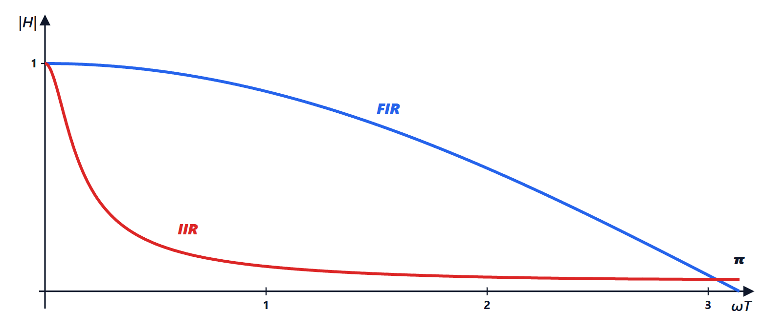
With  ,
 is the frequency response, periodic with period
 and (for real coefficients) symmetric: it is enough to look at it between 0 and the Nyquist frequency
 . The two-sample moving average
 has magnitude
 , zero at Nyquist; the exponential filter
 with
 is a much more selective low-pass, but with feedback (IIR).
A Python example
With the free python-control library (in MATLAB the functions have almost the same names: tf, c2d, step) a system is discretised and the methods are compared:
import control as ct

T = 0.1                                  # sampling period [s]
G = ct.tf([2], [1, 2])                   # G(s) = 2/(s + 2)
Gzoh = ct.sample_system(G, T, method='zoh')
Gtus = ct.sample_system(G, T, method='tustin')
print(Gzoh)                              # 0.1813 / (z - 0.8187)
print(Gtus)                              # (0.09091 z + 0.09091) / (z - 0.8182)
print(ct.poles(Gzoh))                    # [0.8187] = exp(-2*0.1)
The ZOH pole is exactly  ; the Tustin one,
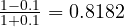 , is very close because
 is small. In MATLAB:
G = tf(2,[1 2]); Gz = c2d(G, 0.1, 'zoh').
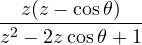
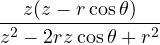
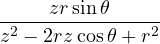
Tables to remember
Transforms (sequences that are zero for )
 |  |
|---|---|
 | 1 |
 |  |
 |  |
|  |
|  |
 |  |
 |  |
 |  |
 |  |
 |  |
Properties:  ;
 ;
 ;
 ;
 ;
 ; initial value
 ; final value
 .
Discretisations
| Method | Substitution | Preserves stability | Notes |
|---|---|---|---|
| ZOH |  | yes, exact | model of the process with D/A |
| Forward Euler |  | no | simple, needs small |
| Backward Euler |  | yes | adds damping |
| Tustin |  | yes | warps frequencies, use prewarping |
| Pole-zero matching | for poles and zeros | yes | gain must be adjusted |
Exercises with difference equations, filters, stability and discretisations are on the exercise page linked at the top.