The Z transform and discrete-time systems
Definition and region of convergence, delay and convolution, difference equations, FIR and IIR filters, stability in the z-plane, the link with Laplace and Fourier, inversion.
Digital systems do not work with continuous signals but with sequences of samples:  , taken at time intervals
 . An audio filter in a DSP chip, a controller in a microcontroller, an equaliser in a modem compute each output from the latest samples. The Z transform does for these systems what the Laplace transform does for continuous ones: it turns difference equations into algebraic equations, defines the transfer function and ties stability to the position of the poles.
Definition
For a sequence  , zero for
 :
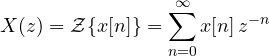
It is a power series in  , so it converges outside a circle: for
 , the region of convergence.
Examples.
- Unit impulse
 (1 for
 , 0 elsewhere):
 .
- Step
 (1 for
 ):
 , for
 .
- Exponential
 :
 , for
 . It is the geometric series, and almost every other transform follows from it.
Properties
- Linearity.
- One-sample delay:
 . It is the key property: is a delay of one sample, and in digital filter block diagrams it is drawn precisely as the symbol , a memory register.
- Advance:
 , the counterpart of the derivative with its initial condition.
- Convolution:
 , with
 .
- Final value:
 , if the limit exists.
Difference equations and the transfer function
A discrete linear time-invariant system is described by a difference equation. Example: a filter taking the weighted average of the new sample and the previous output,

Transforming, with zero initial conditions:  , so

It is the simplest digital low-pass (exponential moving average), the “filter” used in microcontrollers to clean up a sensor reading: with  each new reading weighs 10%. The step response is
 , which tends to 1.
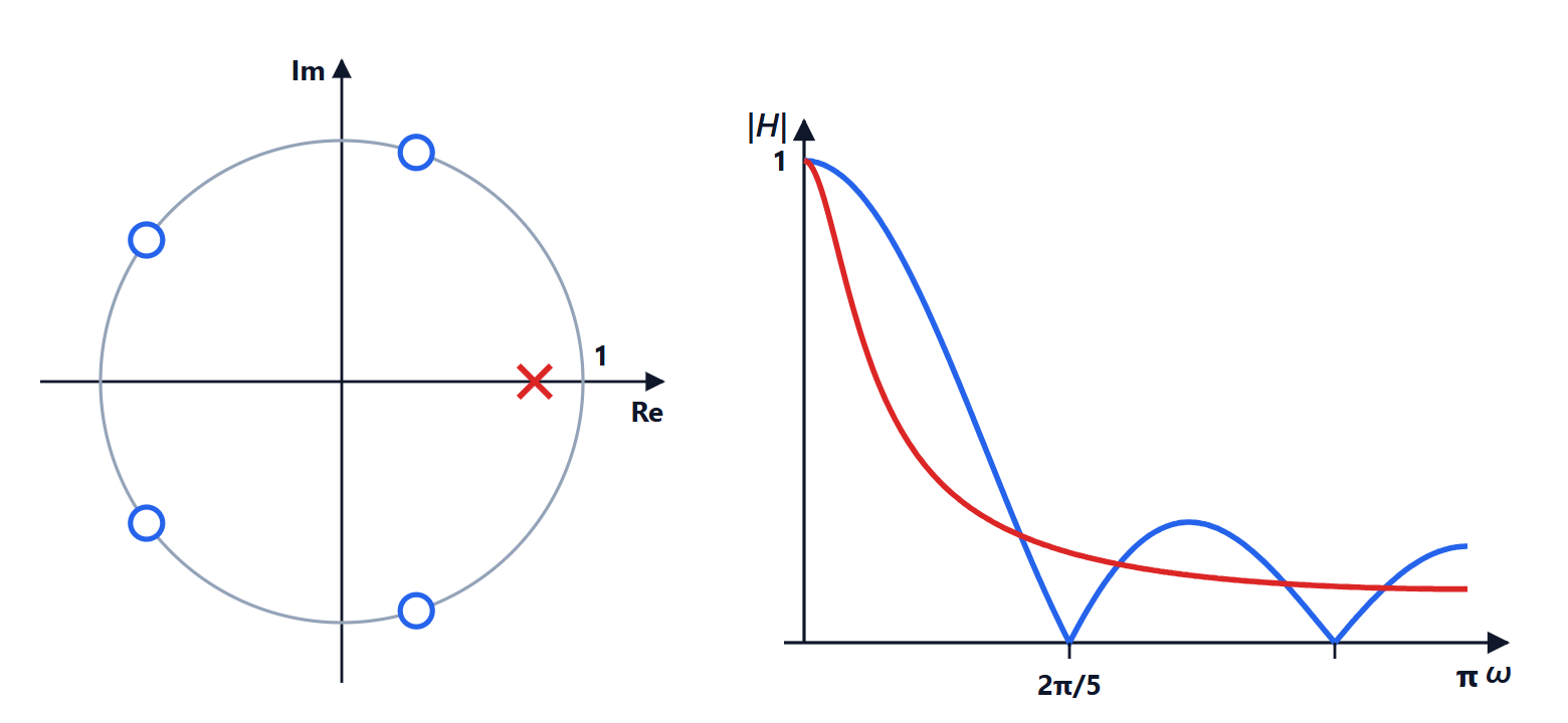
The two big families of digital filters:
- FIR (finite impulse response):
 .
 is a polynomial in : it has poles only at the origin, so it is always stable, and it can have exactly linear phase.
- IIR (infinite impulse response): they also contain terms
 , that is feedback, like the example above. With few coefficients they achieve very selective filters, but they can become unstable.
The z-plane and stability
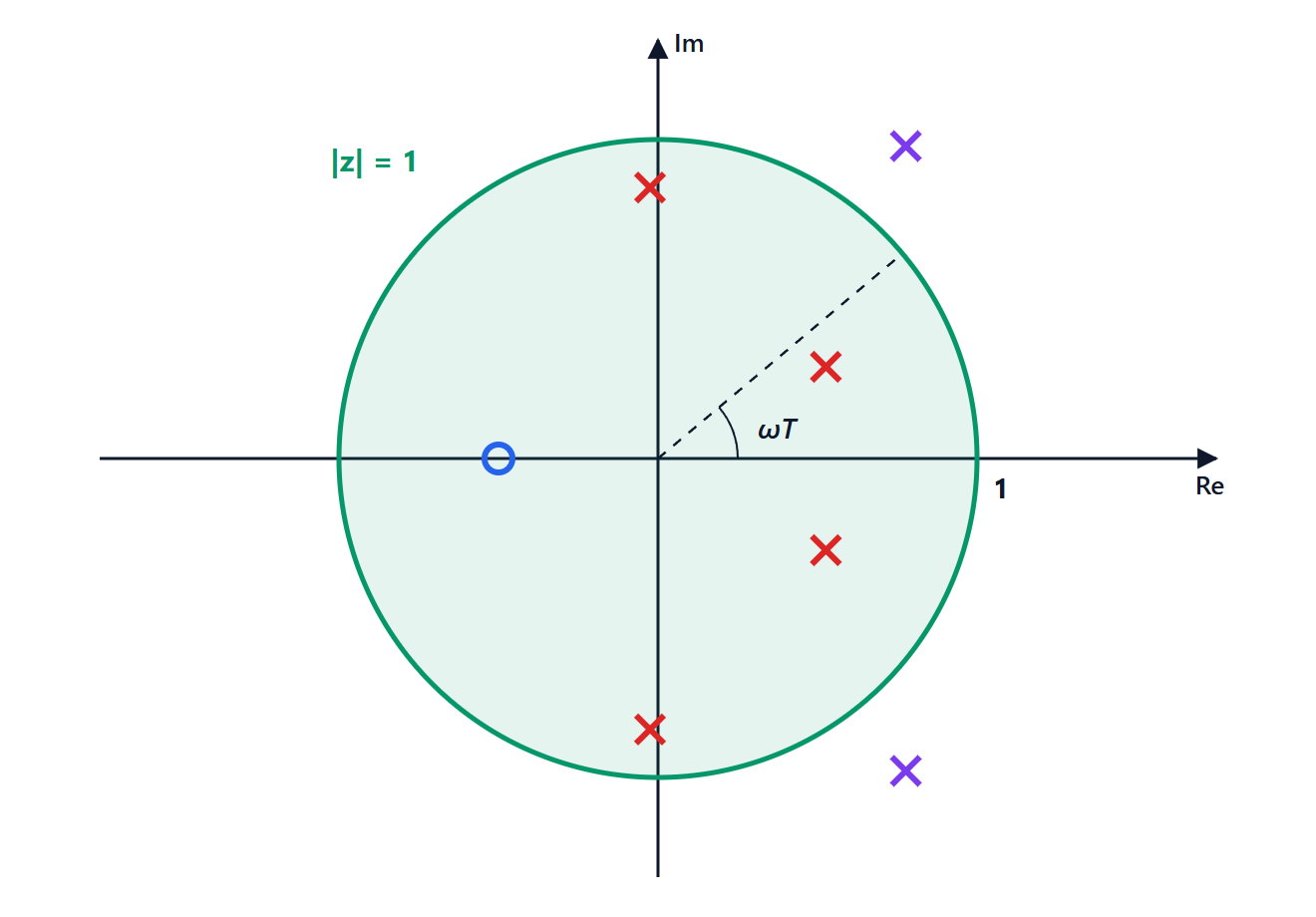
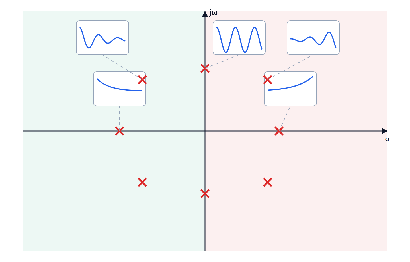
A pole  produces a term
 in the response. If
 the term dies away, if
 it grows. Hence
a discrete system is stable if and only if every pole of its transfer function lies inside the unit circle.
In the example filter the pole is at  : stable for
 . With
 the output would grow by 5% at every sample.
The link with Laplace and Fourier
Sampling a continuous signal with period corresponds to the substitution

The left half of the  plane (
 ) maps inside the unit circle (
 ), the imaginary axis
 maps onto the circle
 . That is why the stability rules correspond: “negative real part” becomes “modulus less than 1”.
Evaluating on the unit circle, , gives the frequency response of the discrete system. One full turn of the circle corresponds to the sampling frequency: the frequency response of a digital system is periodic, which is another way of seeing aliasing. Useful frequencies run from 0 (at  ) to half the sampling frequency (at
 ).
Example. A filter with a zero at , such as 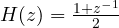 (the average of the last two samples), completely removes the Nyquist frequency: a signal alternating
 gives zero output. It is the simplest FIR low-pass.
Inversion
As with Laplace, partial fractions are used, but it pays to split  , so that the terms become
 , which correspond to . For example

Alternatively you can always divide the numerator by the denominator and read the samples as the coefficients of the series in : exactly what a processor does when it runs the difference equation sample after sample.