Discretising a controller: Euler, Tustin and prewarping
Three approximations of the derivative, Tustin and backward Euler preserve stability (proved), frequency warping proved with an example, prewarping, a discretised PI.
The most common way to obtain a digital controller is to design it in continuous time, with the tools of Automatic Control, and then translate it into a difference equation. This is called design by emulation. The translation is done by replacing  with a function of
 that approximates the derivative, and the choice matters: one method can make a stable controller unstable, another shifts the frequencies. In this lesson we look at the Euler and Tustin methods, the proofs of how they transform the left half-plane, frequency warping with prewarping, and a discretised PI.
Three approximations of the derivative
A derivative can be approximated by the forward difference quotient, the backward one, or by integrating with the trapezoidal rule. In terms of the z-transform, where is a one-step advance:
| Method | Substitution | Inverse |
|---|---|---|
| Forward Euler |  |  |
| Backward Euler |  |  |
| Tustin (trapezoidal, bilinear) | 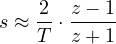 | 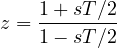 |
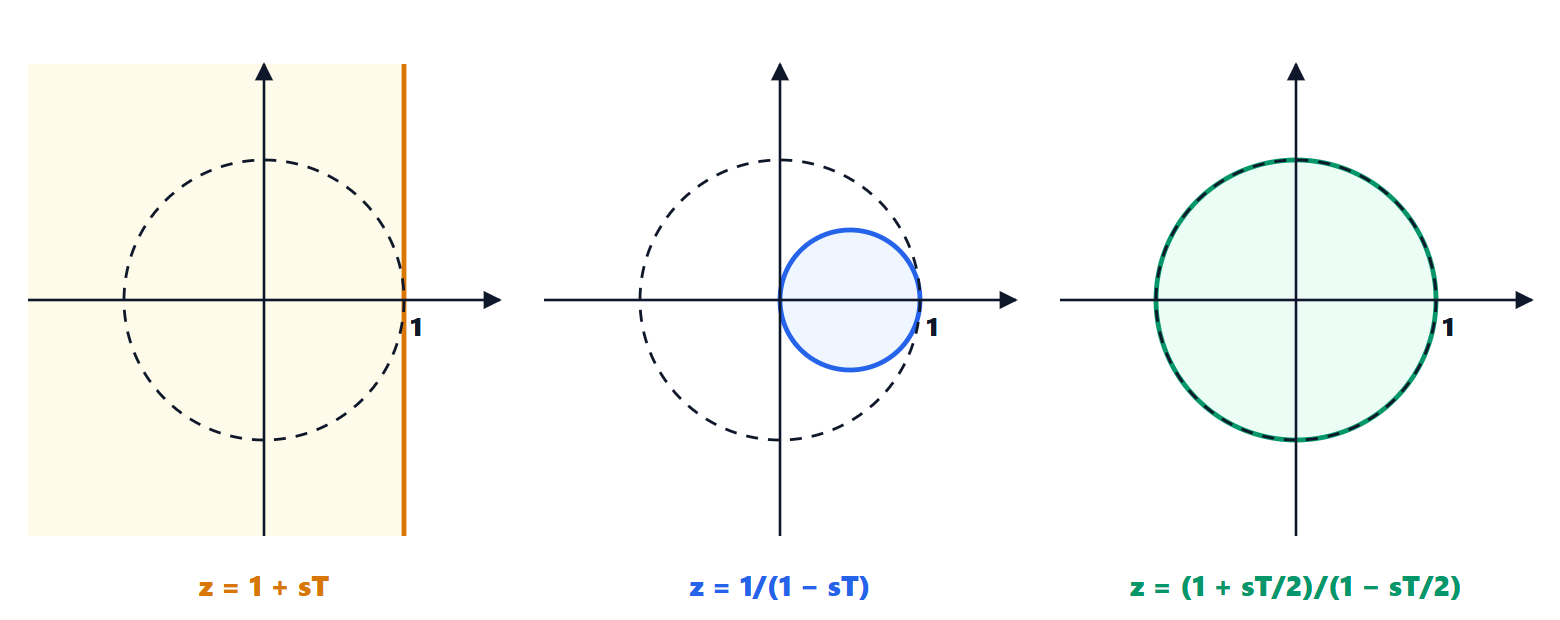
Each method carries the poles of the continuous controller to points of the z-plane. The question is: does a stable pole stay stable?
What happens to stability
Theorem. With the Tustin method a point has negative real part if and only if its image lies inside the unit circle; the imaginary axis goes onto the circle.
Proof. With  and
 ,
 :

The numerator exceeds the denominator by  . So
 if and only if
 , i.e.
 , and
 if and only if
 . ∎
A stable continuous controller thus becomes a stable digital controller, and an unstable one stays unstable: Tustin preserves stability exactly.
Theorem. With backward Euler the left half-plane goes into the circle centred at  with radius .
Proof. From  :

and  if and only if the point
 is closer to
 than to
 , i.e. if . In that case
 . ∎
The small circle lies inside the unit one: a stable controller stays stable, but some unstable controllers become stable too, and the dynamic behaviour is distorted.
With forward Euler, on the other hand, the stable pole  becomes
 , which leaves the circle if
 . A controller with a pole that is fast compared with the period becomes unstable: the method should only be used with periods much smaller than all time constants, and this is the same stability limit as explicit numerical integration (Numerical Calculus lesson on differential equations).
Frequency warping
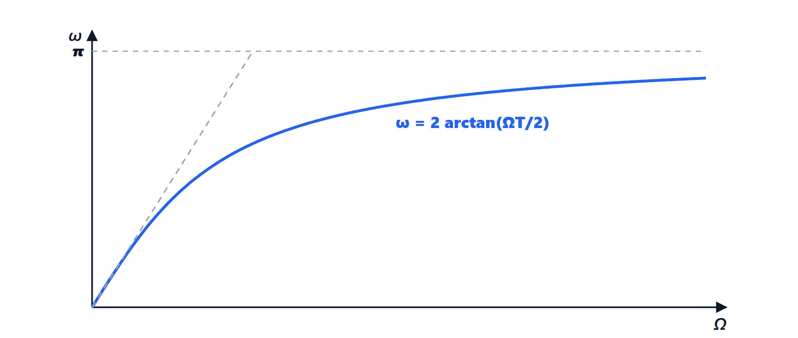
Tustin preserves stability but not frequencies. To see where the imaginary axis ends up, compute the value of corresponding to  :

(factoring  out of numerator and denominator). The digital controller at frequency
 behaves like the continuous one at frequency
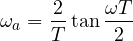
For small  ,
 and
 ; near the Nyquist frequency
 the tangent goes to infinity, and the whole continuous frequency axis is compressed into the interval from 0 to . It is the same frequency warping as in IIR filters (Digital Signal Processing lesson on IIR filters and the bilinear transform).
Example. With  ms, a lead network with its zero at 200 Hz (
 rad/s) ends up, in the digital controller, at frequency
 rad/s, i.e. about 179 Hz: a 10 % error.
Prewarping eliminates the error at a chosen frequency  , the most important one (the zero of the network, the crossover frequency, the frequency of a notch filter):
 is replaced by
 . At frequency the two controllers coincide exactly.
Other methods
- Matched pole-zero: every pole and zero is mapped with
 , and the static gain is adjusted. It preserves pole positions exactly.
- Step invariance: the controller is discretised as if it were a process preceded by a hold (lesson on sampled-data systems).
Whatever method is used, emulation neglects the  delay of the hold and the computation delay, which reduce the phase margin (lesson on implementation). It works well if sampling is fast, 20 to 30 times the closed-loop bandwidth; with longer periods direct design in the z-plane is preferable.
Example: a PI with Tustin
The controller  with the Tustin substitution becomes

Multiplying by  and going back to the time domain ( is a one-step advance), we obtain the algorithm

It is already in incremental form (Process Control lesson on digital control): it computes the change of the command, and lends itself well to limiting the integral action against saturation.