Implementing a digital controller: computation delay, jitter and quantisation
Phase-margin loss due to delay proved with an example, jitter, the dead zone of quantised integral action proved, filter structure, anti-windup and practical rules.
A digital controller designed well on paper can work badly on the microcontroller. Computation takes time, converters have a finite number of levels, arithmetic has limited precision, and the program shares the processor with other tasks. In this lesson we look at computation delay and the proof of its cost in phase margin with an example, timing variability, the effects of quantisation with the proof of a steady-state error that integral action cannot remove, and the practical rules for a robust implementation.
Computation delay
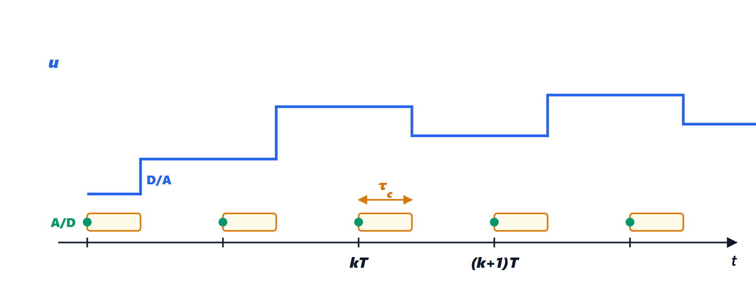
Between sampling the measurement and updating the command, the computation time  elapses. There are two choices:
- update the command as soon as it is ready: the delay is , but it varies from one cycle to the next;
- update it at the next sampling instant: the delay is always a whole period
 , larger but constant and easy to include in the model as a factor
 (lesson on stability in the z-plane, where one step of delay halved the maximum gain).
Theorem. A pure delay  in the loop leaves the magnitude of the loop function unchanged and reduces its phase by
 radians; the phase margin decreases by
 , where
 is the crossover frequency.
Proof. The delay has transfer function  , and in sinusoidal steady state
 , with magnitude 1 and phase
 . Multiplied by the loop function
 , it does not change the frequency at which
 and subtracts from the phase at that point, hence from the margin. ∎
The computation delay adds to that of the hold, about  (Process Control lesson on digital control), and that of the anti-aliasing filter in front of the A/D.
Example. With  rad/s,
 ms and update at the next sample (
 ), the margin loss is
 rad, about 8.6°. With
 ms it would be 86°: the system would almost certainly become unstable.
A simple rule reduces the delay: first compute and write the output, then update the controller state. In most algorithms the output depends on the new measurement through a single product and a sum; all the other computations (updating integrators, filters, diagnostics) are done afterwards, while waiting for the next sample.
Timing variability
If sampling does not happen at exactly regular intervals, or the computation time varies (interrupts, caches, other tasks), the delay fluctuates: this is jitter. The controller is designed for a fixed , and large jitter is equivalent to an extra disturbance and a loss of margin. It is fought by triggering the A/D converter from a hardware timer, not from the program, updating the D/A the same way, and giving the control task the highest priority in a real-time operating system.
Quantisation
An  -bit A/D converter distinguishes
 levels (Signal Theory lesson on quantisation); the D/A and the program’s internal numbers also have a minimum step. In the closed loop quantisation produces non-linear effects: dead zones and limit cycles, small permanent oscillations of one or two steps.
Theorem. Consider an integral action in incremental form  , with the command represented with step
 and the increment rounded to the nearest step. Then a constant error with
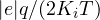 is never corrected.
Proof. If  , rounding
 to the nearest multiple of gives 0: the command does not change, the output does not change and the error stays the same. The situation repeats identically at every step. ∎
Example. A 12-bit command normalised to full scale,  , and
 (slow integral action, fast sampling): the error can remain up to
 , i.e. 12 % of full scale, despite the integral action. The paradox is that sampling faster makes things worse, because it reduces
 .
The remedy is to keep the integrator with more bits than the command (for instance 32 bits, or by accumulating the rounding remainder) and to quantise only at the output towards the D/A. The same problem affects the coefficients: with fast sampling the poles approach  (because
 ) and filter coefficients become numbers like 0.9995 that need many bits. Filter structures matter (Digital Signal Processing lesson on digital filter structures): cascades of second-order sections, or the delta operator
 , which works on the difference between samples.
Other practical rules
- Saturation and anti-windup: the actuator has limits; when the command saturates, the integrator must be stopped or wound back (Automatic Control lesson on the PID controller). In incremental form it is enough to saturate the accumulated command.
- Bumpless transfer between manual and automatic: on engagement the controller is initialised with the current command.
- Fixed-point arithmetic with saturation instead of overflow, which would turn a large positive number into a large negative one.
- Anti-aliasing filter before the A/D, because a high-frequency disturbance, once sampled, folds back to low frequency and the controller tries to correct it.
- Watchdog and plausibility checks: if the program hangs or a measurement is absurd, the actuator must be brought to a safe condition.