Pole placement and deadbeat control
Discrete state model, Ackermann's formula, cancelling the state in n steps proved with Cayley-Hamilton, the double integrator step by step, control effort, integral action.
In state space, digital control has a possibility that does not exist in continuous time: bringing the state exactly to zero in a finite number of steps with a linear control law. This is deadbeat control. In this lesson we look at the discrete state model, pole placement with Ackermann’s formula, the proof that deadbeat control cancels the state in  steps, the complete example of the double integrator, the price paid in control effort and the addition of integral action.
The model and state feedback
The process  ,
 , with the command constant between samples, becomes exactly

(Systems Theory lesson on discrete-time systems). With state feedback  the closed loop is
 . If the system is reachable (lesson on reachability), the eigenvalues of
 can be placed anywhere (Automatic Control lesson on state space). For a single input, Ackermann’s formula gives the gain that achieves the desired characteristic polynomial
 :

A natural choice of poles is  , where the
 are the poles of a good continuous design.
Deadbeat control
All the poles are placed at  .
Theorem. If all the eigenvalues of  are zero, then
 for any initial state, where is the order of the system.
Proof. The characteristic polynomial of  is
 . By the Cayley-Hamilton theorem every matrix annihilates its own characteristic polynomial, so
 . Then
 . ∎
No linear continuous system can do this: the solution is a combination of exponentials, which approach zero without ever reaching it. In discrete time, instead, the nilpotent matrix “switches off” the state in steps, and then keeps it at zero.
Example: the double integrator
With  (a unit mass pushed by a force), state
 :

The deadbeat gain is  . Check:

with trace 0 and determinant 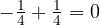 : the characteristic polynomial is
 .
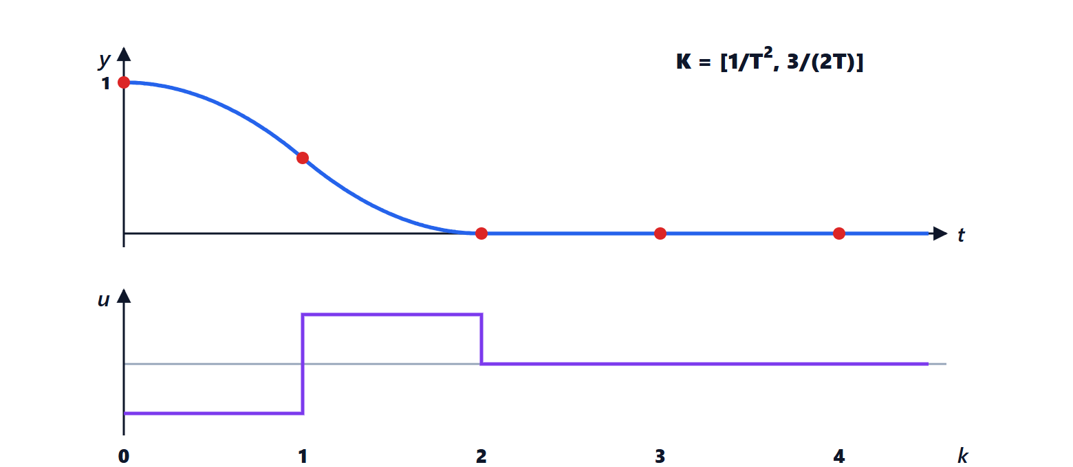
With  and initial state
 : the first command is
 , leading to
 ; the second is
 , leading to
 . The mass is set moving with one push and stopped with an equal and opposite push: the “bang-bang” strategy one would use by hand.
The price
Deadbeat is the fastest possible controller, and there is a price to pay:
- control effort: in the double integrator the gain is proportional to
 . Halving the period, i.e. asking to reach zero in half the time, quadruples the command: with real actuators saturation is reached immediately;
- sensitivity: all the poles at the same point make the system very sensitive to model errors and measurement noise;
- inter-sample oscillations: a deadbeat controller designed on the output rather than on the state can have the samples on the reference while the continuous output oscillates (lesson on sampled-data systems), especially if it cancels model zeros close to
 .
In practice deadbeat is used as a reference limit, or with a period chosen so that the command stays within limits; more often the poles are placed at points close to the origin but distinct, or chosen with optimal control (lesson on LQ and predictive control).
Integral action
State feedback does not cancel the steady-state error in the presence of constant disturbances or model errors. A state integrating the error is added:

and the feedback is designed on the augmented system  , of order
 , with
 . If the augmented system is reachable (the process must not have zeros at
 ), the poles are placed as before, and at steady state a constant
 forces
 .