Stability in the z-plane and the Jury criterion
The z = e^sT mapping proved, the second-order Jury criterion with full proof, sampling and computation delay limiting the gain, discrete Nyquist.
In continuous control a system is stable if the poles have negative real part; in digital control the good region is the inside of the unit circle. The link between the two worlds is the exponential function  , which also explains why sampling makes stability harder. In this lesson we look at the correspondence between the s-plane and the z-plane, the Jury criterion for second order with its full proof, and two examples showing how sampling and computation delay limit the gain.
From the s-plane to the z-plane
A continuous mode  sampled with period
 gives the sequence
 , i.e. a discrete mode with pole

(Systems Theory lesson on discrete-time systems, where we saw that the eigenvalues of  are the exponentials of those of
 ).
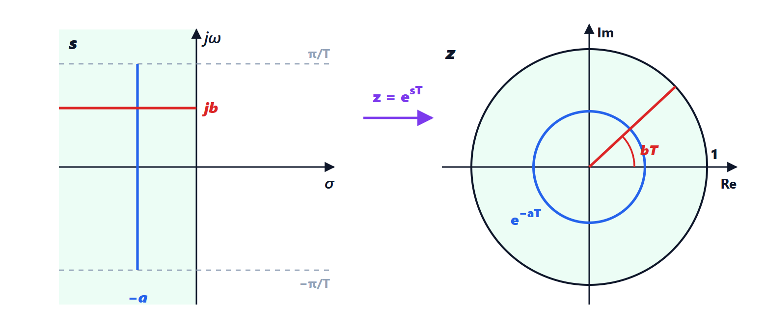
Theorem. The point  has negative real part if and only if lies inside the unit circle.
Proof.  , because
 . And
 if and only if
 . ∎
The same proof says more: vertical lines  constant become circles of radius
 , and horizontal lines
 constant become rays at angle
 . Points differing by
 in
 end up at the same
 : this is aliasing (lesson on the sampling theorem), and the correspondence is one-to-one only in the strip
 .
A linear discrete system is therefore asymptotically stable if and only if all the poles of the closed-loop transfer function have modulus less than 1. The closer the pole is to the origin, the faster the mode dies out; a pole at  corresponds to a mode that vanishes in a single step, with no continuous equivalent.
The Jury criterion for second order
For continuous polynomials there is the Routh criterion; for discrete ones there is the Jury criterion, which decides whether all the roots are inside the unit circle without computing them. For second order it has a very simple form.
Theorem. The roots of  , with real coefficients, both lie inside the unit circle if and only if

Proof. Let  be the roots:
 and
 .
Necessary conditions. If the roots are inside the circle,  . If they are complex conjugate,
 and
 . If they are real and in
 , the factors
 and
 are positive, so
 and
 .
Sufficient conditions. If the roots are complex conjugate,  . If they are real,
 is an upward parabola, positive at
 and at
 : the roots are both in , or both greater than 1, or both less than (if one were below and the other above ,
 would be negative). In the last two cases
 , contradicting the hypothesis. ∎
For higher orders the Jury criterion builds a table similar to Routh’s. Alternatively the bilinear transformation  is used, which maps the inside of the unit circle onto the left half of the
 -plane (lesson on discretisation), followed by the Routh criterion.
Example: sampling limits the gain
Let an integrator,  , be controlled with a proportional action
 . In continuous time the closed loop has pole
 , stable for any
 . Digitally, with the hold,
 (lesson on sampled-data systems), and the characteristic polynomial of
 is

stable if and only if  , i.e.
 . For
 the pole is at zero and the error vanishes in one step; for
 the response is stable but alternating, the sign of a controller that over-corrects; beyond 2 it diverges. The admissible gain is limited by the period: the controller acts “blindly” for a whole period before seeing the effect of its action.
Example: one step of computation delay
If the command computed with sample  is applied only at instant
 (lesson on implementation), the loop also contains a delay
 :
 and the characteristic polynomial is

With  and
 , the Jury criterion requires
 ,
 and
 : the maximum gain has halved, from
 to . At the limit the roots are
 , right on the unit circle: a sustained oscillation with six samples per period.
Frequency response
The Nyquist criterion also holds in discrete time (lesson on the Nyquist criterion):  is plotted for from 0 to
 , i.e. along the unit circle instead of the imaginary axis. Gain and phase margins have the same meaning, and are read on the Bode plots of the discrete loop function, which stop at the Nyquist frequency.





