Direct design in the z-plane: specifications, root locus, steady-state error
Specifications as a region of the z-plane, the constant-damping spiral proved, the discrete root locus with an example, the final value theorem proved, the w-transform.
Instead of designing in continuous time and translating, one can design directly on the discrete model of the process, which is exact at the sampling instants (lesson on sampled-data systems). The advantage is that the delay of the hold and the computation delay are already in the model, and longer sampling periods can be used. In this lesson we look at how response specifications become a region of the z-plane, with the proof of the constant-damping spiral, the discrete root locus with a complete example, steady-state error with the final value theorem, and frequency-domain design.
Specifications in the z-plane
Step-response specifications translate, as in Automatic Control, into conditions on the dominant poles  (lesson on time response): the damping
 sets the overshoot, the real part
 sets the settling time, about
 at 2 %. With
 they become conditions on the z-plane.
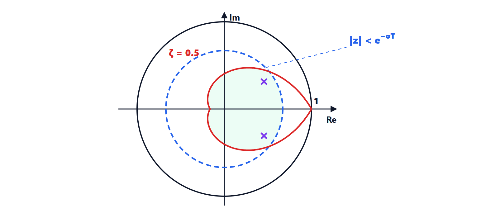
- Settling time:
 , so the poles must lie inside the circle of radius
 .
- Damping: poles with constant lie on a spiral.
Theorem. The discrete poles corresponding to a fixed damping lie on the logarithmic spiral
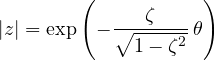
where  is the angle of the pole.
Proof. The pole is  : modulus
 and angle
 . Obtaining
 from the angle and substituting it into the modulus gives the formula. As
 varies, grows and the modulus decreases exponentially: it is a logarithmic spiral starting from
 . ∎
The angle also has a practical meaning:  is the number of samples per period of the oscillation. With small , below
 , there are at least eight samples per oscillation and the behaviour between samples is well represented.
Example. With  s and a settling time of 1 s:
 s
 and
 . With maximum overshoot of 16 %, i.e.
 , the spiral factor is
 . The green region of the figure satisfies both.
The discrete root locus
The characteristic equation  has the same form as in the continuous case, and the root locus is drawn with the same rules (Automatic Control lesson on the root locus): it starts from the poles, ends at the zeros or at infinity, and on the real axis occupies the segments with an odd number of poles and zeros to the right. Only the interpretation changes: the stability boundary is the unit circle, and the good regions are those of the figure.
Example. An integrator with one step of computation delay has  , with poles at 0 and 1 and no zeros. The locus occupies the segment
 ; the two branches meet at the midpoint
 , where the polynomial
 has a double root, i.e. for
 ; then they go up and down along the vertical line
 (the sum of the roots stays 1). They leave the unit circle when the product of the roots
 equals 1, as found with the Jury criterion (lesson on stability in the z-plane). The choice gives a double pole at , equivalent to the continuous pole
 : a fast, non-oscillating response that settles in a few samples.
Steady-state error
As in continuous time, the steady-state error depends on the number of integrators in the loop. In discrete time an integrator is a pole at .
Final value theorem. If the sequence  converges, its limit is

Proof. The transform of the difference  is
 . Evaluating the series that defines it as
 (where the terms
 tend to 1) gives the sum of all the differences, which is
 . So
 . ∎
With the step  and the error
 , the steady-state error is
 : zero if
 has at least one pole at , otherwise
 . The rules on system type (lesson on steady-state errors) hold with in place of
 .
Frequency-domain design
To use Bode plots and continuous compensators (lesson on compensators) the discrete model is transformed with the w-transform:
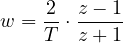
which maps the unit circle onto the imaginary axis (lesson on discretisation). In the w-plane the process, already including the hold and delays, is treated as a continuous transfer function: the compensator is designed with margins and bandwidth, and brought back to  with the inverse substitution, without further approximations. The w-plane frequency
 and the true one are related by the tangent,
 , to be kept in mind in the specifications.