Drives: motion profile, gear ratio and sizing
Trapezoidal profile times proved with an example, S-curves, the optimal gear ratio proved, RMS torque for thermal sizing, cascaded controllers.
Conveyors, robots, packaging machines, machine tool axes: almost every movement in a factory is produced by an electric motor controlled by a drive (an electronic converter with its control, Power Electronics lessons). Designing an axis means choosing the motion profile, the motor, the gearbox and the controllers. In this lesson we look at the trapezoidal profile with the time formulas proved and an example, the optimal gear ratio with its proof, RMS torque for thermal sizing, and the structure of cascaded controllers.
The motion profile
To move a load over a distance  in minimum time, with maximum velocity
 and maximum acceleration
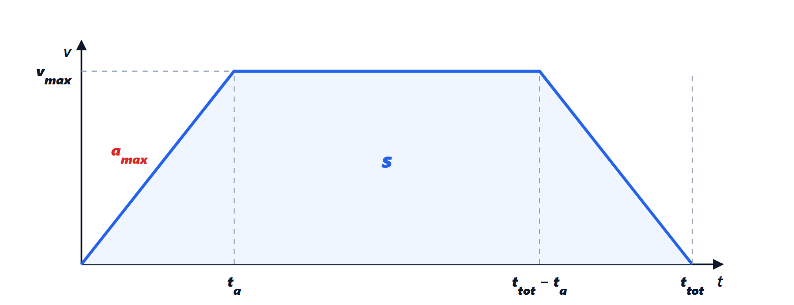
 , one accelerates at maximum, continues at constant velocity and brakes at maximum: the trapezoidal profile.
Theorem. If  , the total time is
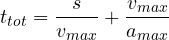
otherwise maximum velocity is not reached, the profile is triangular and  .
Proof. Acceleration lasts  , and braking the same. The displacement is the area of the trapezoid:
 (mean of the bases times the height), hence
 . The constant-velocity segment exists if
 , i.e.
 , i.e. . Otherwise one accelerates up to half way and brakes: each half
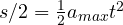 lasts
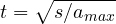 . ∎
Example.  m,
 m/s,
 m/s²:
 , so
 s. For short moves acceleration matters, for long ones velocity.
The trapezoidal profile has stepped acceleration: the jerk (the derivative of acceleration) is infinite and makes the mechanics vibrate. S-curve profiles, with ramped acceleration, limit jerk at the price of a slightly longer time, and are the norm where precision and absence of vibration matter.
The gear ratio
Between motor and load there is often a gearbox: the motor turns  times faster than the load and the torque reaches the load multiplied by (neglecting losses). Which ratio makes the motion fastest?
Theorem. With a motor of torque  and inertia
 and a load of inertia
 , the load acceleration is maximum with the gear ratio

i.e. when the load inertia referred to the motor,  , equals the motor’s.
Proof. If the load accelerates by  , the motor accelerates by
 . The motor supplies torque to accelerate itself and the load referred to the motor shaft:
 . Hence
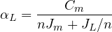
The denominator, as a function of , has derivative 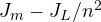 , zero for
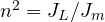 , where it is minimum (it is the sum of a term increasing and one decreasing in , with constant product). ∎
Example.  kg m²,
 kg m²:
 . In practice a ratio close to the optimum is chosen consistently with the motor’s maximum speed, and an inertia ratio ( over ) not too far from 1 also makes the system easier to tune, because the elastic mechanics between motor and load disturbs the speed loop less.
Thermal sizing
A motor heats up with copper losses, proportional to the square of the current and hence of the torque. In a duty cycle with torques  for times
 , what counts is the RMS torque
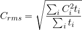
which must be below the motor’s continuous rated torque (the thermal time constant, minutes, is much longer than the cycle). The peak torque must instead stay below the maximum torque. Example. A 1 s cycle with 0.2 s at 10 N m (acceleration), 0.5 s at 2 N m, 0.2 s at 6 N m (braking, with the load helping), 0.1 s at rest:  N m. A motor of at least 5.4 N m continuous and 10 N m peak is needed; the mean value, 4.2 N m, would lead to undersizing it.
Cascaded controllers
A servo drive has three nested loops (Process Control lesson on cascade control):
- the current (torque) loop, the innermost and fastest, with a bandwidth of a few kilohertz, exploiting the motor’s vector control (Power Electronics lesson on inverters);
- the velocity loop, with a bandwidth of a few hundred hertz, usually a PI;
- the position loop, the outermost, often proportional with velocity and acceleration feedforward computed from the profile.
Each loop must be 3 to 10 times slower than the inner one, which can thus be seen as almost ideal. Feedforward is decisive: with the profile known in advance, the controller already applies the torque needed to accelerate the inertia, and the position loop only has to correct errors, not chase the reference.
When several axes must move together (electronic cams, trajectory interpolation, a robot), the motion controller computes the references of all axes in synchrony, over a deterministic network such as EtherCAT (lesson on industrial networks).





