Sensors and connections: the 4-20 mA loop and encoders

An automated system sees the plant through sensors and acts through actuators; the link between the field and the controller must carry signals over hundreds of metres, in environments full of noise, and report its own faults. In this lesson we look at the 4-20 mA current loop with the voltage budget proved and an example, scaling and the “live zero”, sensor parameters, and incremental and absolute encoders with the proofs on quadrature decoding and Gray code.

The 4-20 mA current loop

The most widespread standard for analogue field signals transmits the measurement as a current between 4 and 20 mA, proportional to the value between the minimum and maximum of the range.

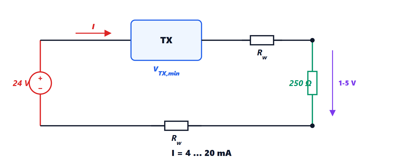
Why a current and not a voltage? In a series circuit the current is the same at every point (Kirchhoff’s current law): the wire resistance, which changes with length and temperature, does not alter the measurement, whereas a voltage would arrive reduced by the drop across the wires. Moreover, the low impedance of the circuit makes it insensitive to capacitive disturbances (Electromagnetic Compatibility lesson on coupling). And two wires are enough, carrying both the transmitter’s supply and the signal.

The measured value is obtained with . The zero of the range corresponds to 4 mA, not 0: this is the live zero. A current below about 3.6 mA (broken wire, failed transmitter) or above 21 mA (short circuit) is outside the range and is recognised as a fault (NAMUR recommendation NE 43). With a zero at 0 mA a cut wire would look like a valid minimum reading: for example an empty tank, while it is overflowing.

Theorem. A loop supplied with voltage , with a transmitter needing at least to operate, works over the whole range if the total loop resistance (wires plus measuring resistor) satisfies

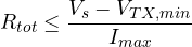
Proof. By Kirchhoff’s voltage law, the voltage available across the transmitter is . It is minimum when the current is maximum, mA (or a little more if the high fault must be signalled). It must remain at least : , hence the formula. ∎

Example. V, V: Ω. With 250 Ω of measuring resistance, 350 Ω remain for the wires: with 0.5 mm² cable (about 36 Ω/km per conductor, i.e. 72 Ω/km out and back) almost 5 km can be reached. If other instruments are inserted in the loop (a local indicator, an intrinsic safety barrier for explosive areas), each uses part of the budget.

On top of the analogue current the HART protocol superimposes a frequency-modulated digital signal with zero mean, which does not disturb the measurement and allows the transmitter to be configured and its diagnostics read. More and more often sensors are connected directly to a network (IO-Link, fieldbuses, lesson on industrial networks).

Sensor parameters

• Measuring range and permissible overload.
• Accuracy: how close the measurement is to the true value, including all errors (Electrical Measurements lesson on uncertainty).
• Repeatability: how similar repeated measurements under the same conditions are. For many control loops it matters more than accuracy, because a constant error is compensated.
• Resolution: the smallest detectable change.
• Response time, often expressed as a time constant: a slow sensor adds a delay to the control loop (lesson on process models).
• Ingress protection (IP), operating temperature, certifications for explosive atmospheres (ATEX).

Encoders

An incremental encoder measures a rotation with a disc with lines read by two sensors offset by a quarter of a line: the signals A and B are two square waves in quadrature.

Theorem. Counting all edges of A and B gives counts per revolution, and the direction of rotation follows from the order of the edges.

Proof. In one line period each wave has one rising and one falling edge; the edges of A and B, offset by a quarter period, never coincide, and in one period there are four, equally spaced. With periods per revolution there are edges. Rotating one way A leads B by a quarter period, the other way it lags: at the rising edge of A, B is 0 in one direction and 1 in the other, and the counter goes up or down accordingly. ∎

Example. A 1024-line encoder gives 4096 counts per revolution, i.e. a resolution of about 0.088°. A third signal Z (index) gives one pulse per revolution, to find zero.

An incremental encoder loses its position when switched off. An absolute encoder reads on several tracks a code identifying the position. Gray code is used, in which consecutive positions differ by a single bit: with natural binary, going from 0111 to 1000 four bits change, which the sensors never read at exactly the same instant, and for a moment any value could be read. Gray code is built by reflection: the -bit code is the -bit one preceded by 0, followed by the same in reverse order preceded by 1. By induction, consecutive positions within each half differ by one bit (by the hypothesis on the -bit code), and at the boundary between the halves the two words have the same tail and differ only in the added bit; the first and last also differ by a single bit, and the code is cyclic.