Acceptance tests, commissioning, OEE and maintenance

A plant is not finished when the last cable is connected: it must be tested, started up, handed over and then kept efficient for years. In this lesson we look at factory and site acceptance tests, virtual commissioning with the digital twin, operator interface design and alarm management, the OEE indicator with the proof of its compact form and an example, and maintenance strategies.

Acceptance tests

• FAT (factory acceptance test): the customer checks the machine or the panel at the manufacturer’s premises, before shipment, following a written test protocol that traces back to the requirements (lesson on architecture). Fixing an error here costs much less than on site.
• SAT (site acceptance test): after installation, the tests are repeated in the real plant, with the real connections, and those that can only be done there are added.
• Commissioning: point-by-point wiring checks (every sensor, every actuator), instrument calibration, dry runs of the sequences and then runs with product, loop tuning, tests of the safety functions.
• Documentation handed over: updated electrical diagrams, programs with source code, operation and maintenance manuals, certificates, declaration of conformity.

Virtual commissioning

On-site commissioning is expensive and under pressure: the plant must start, and every day of delay is lost production. Virtual commissioning connects the real PLC program to a simulation model of the plant (machine kinematics, sensors, actuators, flow of parts), and tests the software before the hardware exists. Sequence errors, missing interlocks and collisions between axes are found this way. The same model, kept aligned with the plant and fed with its data, becomes the digital twin, useful for training operators, trying out changes and optimising production.

The operator interface

The human-machine interface (HMI) must show at a glance whether all is well, and draw attention only when needed. The ISA-101 standard recommends sober graphics, with grey backgrounds and few colours, reserving bright colours for abnormal conditions: on an all-colourful screen a red alarm goes unnoticed. Screens are organised in levels, from the plant overview to the details of a piece of equipment, with trends of the important quantities.

Alarm management (ISA-18.2, IEC 62682) starts from a principle: every alarm must require an operator action. A system generating hundreds of alarms an hour, many without consequences, teaches people to ignore them, and in a real emergency the important information is lost in the flood (this was a factor in several serious industrial accidents). Indicative targets are a few alarms per operator per hour in normal conditions, and alarm rationalisation (removing duplicates, setting priorities, hysteresis and delays) is a real design task.

Overall effectiveness

The MES (lesson on architecture) measures performance with OEE (overall equipment effectiveness), the product of three factors:

• availability = run time / planned time (losses from breakdowns, changeovers);
• performance = (parts produced × ideal cycle time) / run time (losses from minor stops and reduced speed);
• quality = good parts / parts produced (scrap and rework).

Theorem. .

Proof. Multiplying the three definitions, the run time cancels between and , and the parts produced between and :

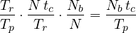
where are the parts produced and the good ones. ∎

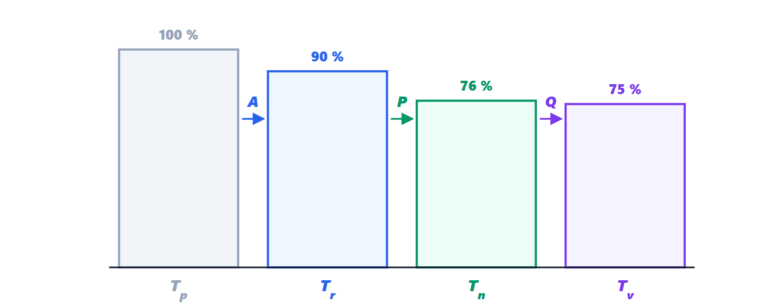
The compact form has a clear interpretation: OEE is the fraction of planned time that would have sufficed to produce the good parts at ideal speed. Example. A 480 min shift, 48 min of stoppages: . Ideal cycle time 0.5 min, 734 parts produced: . 719 good parts: . OEE . A value of 85 % is considered excellent for discrete manufacturing; many plants are between 40 and 60 %. The breakdown shows where to act: here the biggest loss is in performance (minor stops), not breakdowns.

Maintenance

• Corrective: repair when it breaks. Acceptable for cheap, non-critical components.
• Preventive: replace at fixed intervals, before the expected failure. It wastes useful life and does not avoid random failures, which for electronics are the majority (the flat part of the bathtub curve, Microelectronics lesson on testing).
• Predictive (condition-based): the condition of components is measured (bearing vibration with spectral analysis, temperatures, motor currents, valve stroke times) and action is taken when the trend announces a failure. The data are already in the automation system, and automatic analysis, including machine learning techniques, is one of the most concrete applications of Industry 4.0.

The common goal is to increase availability (lesson on architecture) by reducing both failures and repair times.