LQ optimal control and model predictive control
The linear quadratic regulator with the Riccati equation proved by dynamic programming, a closed-form scalar example, LQG, predictive control with receding horizon and constraints.
Pole placement leaves a question open: where to put the poles? Faster means larger commands, slower means errors that last longer. Optimal control answers by writing the trade-off as a cost to be minimised, and predictive control extends the idea to the constraints every real plant has: saturating actuators, temperatures and pressures not to be exceeded. In this lesson we look at the discrete linear quadratic (LQ) regulator with the derivation of the Riccati equation, a scalar example solved in closed form, and predictive control with the receding horizon, constraints and its applications.
The linear quadratic regulator
For the system  we look for the command sequence that minimises

with  positive semidefinite (how much the error weighs) and
 positive definite (how much the command weighs). Increasing relative to asks for a more “frugal” controller.
Theorem. The optimal solution is a state feedback  with

where  is the symmetric positive definite solution of the algebraic Riccati equation

and the minimum cost starting from  is
 .
Proof (dynamic programming). Let  be the minimum cost starting from . By Bellman’s principle of optimality, the optimal first step minimises the cost of the step plus the minimum cost from the next state:

Try  . The quantity in brackets is quadratic in
 ; its gradient with respect to is
 , and setting it to zero:

It is a minimum because the matrix  is positive definite. Substituting , all the terms are of the form
 , and the equality holds for every if and only if satisfies the Riccati equation. ∎
If  is reachable and the state is “seen” by the cost (
 observable), the solution exists, is unique and the closed loop is asymptotically stable. In practice the equation is solved numerically, with a single instruction in computing packages.
Example: an integrator
Take  , with
 and
 . With
 the Riccati equation becomes

and  , with closed-loop pole
 .
 | |  | pole  |
|---|---|---|---|
| 0 | 1 | 1 | 0 (deadbeat) |
| 1 | 1.618 | 0.618 | 0.382 |
| 10 | 3.70 | 0.270 | 0.730 |
| 100 | 10.5 | 0.095 | 0.905 |
With a free command ( ) the optimum is deadbeat (lesson on deadbeat control); with an expensive command the controller becomes slower and slower. For
 the golden ratio appears,
 . The designer no longer chooses the poles, but the weights, which have a direct physical meaning. Continuous LQ control also has guaranteed margins (infinite gain margin, at least 60° of phase); in discrete time the margins are somewhat smaller but remain good.
Together with the Kalman filter (lesson on observers) the LQ regulator forms LQG control, optimal when disturbances and noise are Gaussian, and thanks to the separation principle the two are designed independently.
Predictive control
The LQ regulator knows nothing about limits: if the optimal command exceeds the actuator’s saturation, it is simply clipped, and optimality and sometimes stability are lost. Predictive control (MPC, model predictive control) puts the constraints inside the problem.
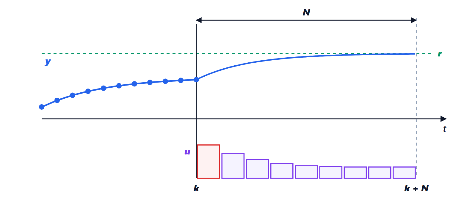
At every sample the controller:
- measures (or estimates with an observer) the current state;
- using the model, predicts the evolution of the output over the next
 steps as a function of the future command sequence
 ;
- chooses the sequence that minimises a quadratic cost (error from the reference plus command effort) while respecting the constraints: limits on commands, on their rate of change, on outputs and on states;
- applies only the first command, discards the others, and at the next sample repeats everything with the new measurement.
Step 3 is a quadratic programming problem: quadratic cost, linear constraints, a unique solution that efficient algorithms find in microseconds or milliseconds. Step 4, the receding horizon, makes the scheme a true feedback: model errors and disturbances are corrected at every cycle.
Some properties:
- with no active constraints, predictive control is a fixed linear feedback; with an infinite horizon it coincides with the LQ regulator;
- stability is guaranteed by adding a terminal cost equal to the LQ cost of the final state, and possibly a terminal constraint;
- it knows reference changes and measurable disturbances in advance, and can start reacting before they occur;
- it naturally handles systems with many coupled inputs and outputs (Process Control lesson on multivariable systems).
Predictive control was born in the late 1970s in refineries, where processes are slow and there is time to compute, and today it is the standard for advanced process control. With modern processors it has reached fast systems: engine management and autonomous driving in cars, drones, power converters and traction electronics, where the “finite control set” version directly chooses the state of the switches (Power Electronics lessons).





