Sampled-data systems: the process as seen by the computer
The digital control loop, the transfer function with a zero-order hold proved, first order, integrator and double integrator, sampling zeros, inter-sample behaviour.
Today almost every controller is a program: a microcontroller reads the measurements with an analogue-to-digital converter, computes the command and sends it to the actuator with a digital-to-analogue converter. The process, however, remains continuous. A system in which continuous signals and sequences of samples coexist is called sampled-data, and designing it requires a model that brings them together. In this lesson we look at the digital control loop, the discrete transfer function of the process as seen by the computer with its proof and three examples, the zeros introduced by sampling and what happens between one sample and the next.
The digital control loop
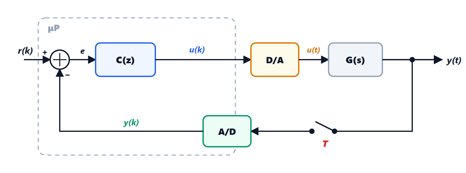
Every  seconds the A/D converter samples the output, the program computes
 and the D/A converter holds it constant until the next update: this is the zero-order hold (ZOH), already seen in the Process Control lesson on digital control, where it was shown that at low frequencies it is equivalent to a delay of
 and how is chosen.
The computer sees only sequences: going out and  coming in. The natural tools are therefore the z-transform and difference equations (Signal Theory and Systems Theory lessons on discrete-time systems). The controller is a transfer function
 ; what is needed is the discrete equivalent of the process, i.e. the function relating the sequence to the sequence
 .
The transfer function with the hold
Theorem. If the process has transfer function  and is preceded by a zero-order hold, the discrete transfer function from to is

where  is the z-transform of the samples
 of the process step response
 .
Proof. The system from to is linear and time-invariant in discrete time, so its transfer function is the z-transform of the response to the unit impulse  ,
 for
 . With this input the hold produces a rectangle of height 1 and width , i.e. a step at time 0 minus a step at time . By linearity the process responds with
 , and the samples are
 . The second term is the first one delayed by one step, and a one-step delay in the z-transform is a multiplication by
 . So the transform of the samples is
 times the transform of , and the Laplace transform of
 is
 . ∎
The model is exact at the sampling instants: there is no approximation, unlike the methods that approximate derivatives.
Three examples
First order. With  we have
 , hence
 and

Multiplying by  :

The continuous pole  has become the discrete pole
 , and the static gain
 is unchanged, as in exact state-space discretisation (Systems Theory lesson on discrete-time systems).
Integrator. With  the step response is the ramp
 , with transform
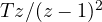 . So
 : the command accumulates, multiplied by the period.
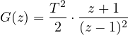
Double integrator. With 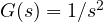 (a mass pushed by a force, a rotating satellite) we have
 , with transform
 , and
Sampling zeros
The last example shows an important fact: the continuous process  has no zeros, but its discrete equivalent has a zero at
 . Sampling creates zeros that the continuous process does not have. A process with
 poles and no zeros generally becomes a discrete system with
 zeros. For small periods these zeros tend to values that depend only on the relative degree, and from relative degree 3 upwards at least one lies outside the unit circle: the discrete model is non-minimum-phase even if the continuous process is not. So not all the zeros of the model can be cancelled by the controller’s poles, as we will see in the lesson on deadbeat control.
What happens between samples
The z-domain model describes the output only at the instants  . Between one sample and the next the output can do things the computer does not see:
- hidden oscillation (inter-sample ripple), typical of very aggressive controllers: the samples sit on the reference, but the continuous output oscillates;
- pathological sampling: if an oscillating mode of the process has frequency
 with
 a multiple of
 , its samples make it look constant or alternating, and the sampled system can lose the reachability or observability that the continuous system had.
For this reason the design is always checked with a continuous simulation of the process too, and the period is chosen with a generous margin: from 10 to 30 samples per closed-loop rise time.





