IIR filters: analogue prototypes and the bilinear transform
The Butterworth filter and the order formula proved, Chebyshev and elliptic filters, the bilinear transform with proof, prewarping, a complete numerical example, impulse invariance, FIR or IIR.
IIR filters have an infinite impulse response because they use feedback: the output also depends on past outputs. With few coefficients they achieve very steep transitions, but they give up linear phase and must be made stable. The classic way to design them is to start from an analogue prototype, one of the filters studied for decades for circuits, and transform it. In this lesson we look at the Butterworth filter with the order formula proved, the bilinear transform with the proof of its properties, frequency prewarping, impulse invariance and a complete numerical example.
Analogue prototypes
The Butterworth filter of order  has
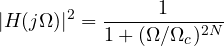
It is maximally flat: at  the first
 derivatives of the squared magnitude are zero, and the gain falls monotonically. At
 it is
 dB, and beyond it falls by
 dB per decade. The poles lie on a semicircle of radius in the left half-plane.
Theorem. To have at most  dB of attenuation up to
 and at least
 dB from
 , the Butterworth order must be

Proof. The attenuation in dB is  . The two conditions give
 and
 . Dividing the second by the first, disappears:
 , and taking logarithms gives the formula. ∎
The Chebyshev type I filter accepts ripple in the passband, type II in the stopband, and the elliptic (or Cauer) filter in both: for the same order it has the steepest possible transition, but the most irregular phase.
The bilinear transform
To go from the analogue filter  to the digital one, substitute
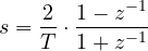
where  is the sampling period. It is the trapezoidal rule applied to the integrator
 , and it turns a rational function into another rational function of the same order.
Theorem. The bilinear transform maps the imaginary axis  onto the unit circle, with
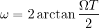
and the left half-plane inside the unit circle. So a stable analogue filter becomes a stable digital filter.
Proof. Inverting the formula,  . For numerator and denominator are complex conjugates,
 , so
 and
 with
 . For
 the point
 is closer to
 than to
 , so
 and
 : the poles end up inside the circle. ∎
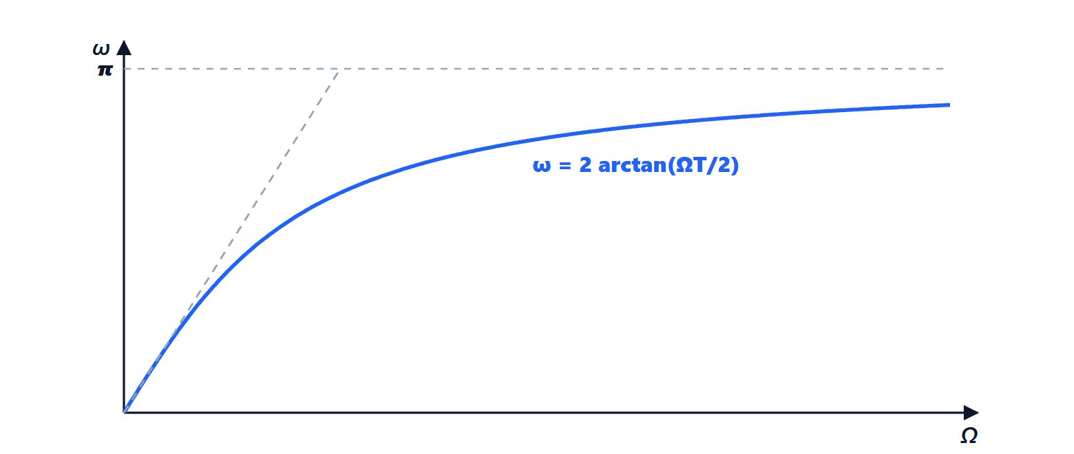
There is no aliasing, because the whole  axis from 0 to infinity is “squeezed” into the interval from 0 to
 . The price is frequency warping: the relation is not linear, and the characteristic frequencies of the prototype end up in the wrong place.
Prewarping
The remedy is to design the analogue prototype with prewarped frequencies: to get a digital cutoff at  , use
 . The critical frequencies then fall exactly where they are needed; the shape of the response between one critical frequency and the next is slightly distorted, but for piecewise-constant filters (low-pass, high-pass, band-pass) it does not matter.
A complete example
We want a second-order Butterworth filter with digital cutoff  (for instance 1 kHz with 10 kHz sampling). With
 prewarping gives
 , and the prototype is
 . Applying the substitution and setting
 , with
 :

The DC gain ( ) is
 , as it must be, and the gain at
 (
 ) is zero, because the numerator
 vanishes: the bilinear transform maps the prototype’s zero at infinity exactly to the Nyquist frequency. The poles have magnitude
 : well inside the circle.
Impulse invariance
An alternative method samples the prototype’s impulse response:  . It preserves the shape of the time response and the linear relation between frequencies, but the digital frequency response is the sum of copies of the analogue one, so there is aliasing: it works well only for low-pass and band-pass filters strongly attenuated before the Nyquist frequency, and it is not used for high-pass filters.
FIR or IIR?
IIR filters reach steep transitions with a much lower order, hence fewer multiplications and less delay: they are the natural choice when phase does not matter, as in many audio filters, equalisers and control loops. FIR filters have exact linear phase, are always stable and tolerate finite precision better: they are preferred in digital communications, imaging and multirate systems. IIR filters are almost always implemented as a cascade of second-order sections, like the one in the example (lesson on structures).