Adaptive filters: Wiener, LMS and noise and echo cancellation
Normal equations and the orthogonality principle proved, the LMS algorithm as gradient descent, the convergence condition proved, normalised LMS, noise and echo cancellation, equalisation.
The filters seen so far have fixed coefficients, computed once from the specifications. But often the signal and the disturbance change over time, or are not known in advance: the echo of a phone call depends on the room, a modem’s channel changes with the line, the noise of an engine with its speed. An adaptive filter updates its own coefficients at every sample to minimise an error. In this lesson we derive the Wiener filter with the orthogonality principle, the LMS algorithm as gradient descent with the proof of the convergence condition, the normalised version and the applications.
The problem
An FIR filter with coefficients  receives the vector of the last
 input samples
 and produces
 . There is a desired signal
 , and the error is
 . We look for the coefficients that minimise the mean squared error
 .
The Wiener filter
Expanding the square, with the input autocorrelation matrix 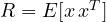 and the cross-correlation vector
 :

It is a quadratic function of the coefficients, a “bowl” with a single minimum.
Theorem. The optimal coefficients satisfy the normal equations  , and at the optimum the error is uncorrelated with every input sample:
 .
Proof. The gradient of  with respect to
 is
 . The minimum of a convex quadratic function (
 is positive semidefinite) is where the gradient vanishes,
 . Moreover
 , which is zero at
 . ∎
The second result is the orthogonality principle: the optimal error no longer contains anything that can be predicted from the input. The Wiener filter, however, requires knowing and  and solving a linear system, and if the statistics change one has to start again.
The LMS algorithm
The idea of Widrow and Hoff (1960) is to go down the gradient one step at a time, using instead of the true gradient, which would require statistical averages, its instantaneous estimate. Replacing and with  and
 , the estimated gradient is
 , and the descent step becomes

with the step size  (the factor 2 is absorbed into ). Each coefficient is corrected in proportion to the error and to the input sample it multiplies. The cost is about
 multiplications per sample: the same order as the filter.
Convergence
Theorem. With stationary inputs, independent from one step to the next, the LMS coefficients converge in the mean to the Wiener solution if and only if

where  is the largest eigenvalue of .
Proof. Let  be the deviation from the optimum. Taking the mean of the update, with the independence assumption
 , gives
 , i.e., using
 ,

is symmetric,  with
 orthogonal; in the coordinates
 the components evolve separately as
 . They tend to zero if and only if
 for every
 , i.e.
 ; the most restrictive condition is that of the largest eigenvalue. ∎
In practice the estimate  , easy to measure, is used:
 . The convergence speed, instead, is set by the smallest eigenvalue: if the eigenvalues are very different (a very coloured input), LMS converges slowly along some directions. A large converges quickly but leaves the coefficients “jittering” around the optimum (the misadjustment, an excess error); a small is accurate but slow to track changes.
Normalised LMS
If the input power varies, a fixed becomes too large or too small. NLMS divides the step by the current energy of the samples:

with a small  to avoid division by zero. It is the version used almost always, for instance in echo cancellers. More expensive algorithms such as RLS (recursive least squares) converge much faster at the price of
 operations per sample, and the Kalman filter is their generalisation to systems described in state space.
Applications
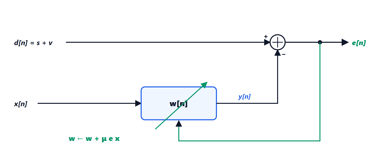
- Noise cancellation. One microphone picks up voice plus noise, a second one picks up only the noise (the reference). The filter learns the transformation between the two noises and subtracts it: by the orthogonality principle the minimum error is exactly the voice, which is uncorrelated with the reference. Active noise-cancelling headphones use a variant of this.
- Echo cancellation. In speakerphones and video calls the loudspeaker leaks back into the microphone. The filter, with the far-end voice as reference, estimates the echo path in the room (hundreds of milliseconds, thousands of coefficients) and removes it.
- Equalisation. In a modem or a radio receiver, the filter compensates the channel distortion by learning from a known sequence, then keeps tracking using the receiver’s decisions.
- Identification. Placed in parallel with an unknown system, with the same input, the filter converges to its impulse response: it is used to measure acoustics, channels and processes.





