Optimal FIR filters: equiripple, Parks-McClellan and linear-phase types
The tolerance mask, the minimax criterion and the alternation theorem, the Parks-McClellan algorithm, order estimation, the four types of linear-phase FIR filters with proof, zeros in quadruples, minimum phase.
The window method is simple but wastes taps: the error is concentrated near the transition and elsewhere the filter does much better than needed. Optimal filters spread the error evenly and meet the same specifications with fewer taps. In this lesson we look at how specifications are written, the minimax criterion and the alternation theorem, order estimation, the four types of linear-phase FIR filters with the proof of their constraints, and the structure of the zeros.
Specifications
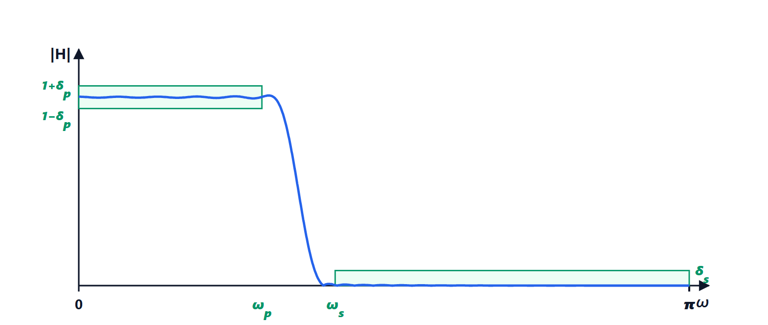
A real filter is specified with a tolerance mask: in the passband ( ) the gain must lie between
 and
 ; in the stopband (
 ) it must stay below
 ; in the transition band between the two nothing is required. In decibels, the passband ripple is
 and the attenuation
 .
The minimax criterion
For a symmetric FIR filter the response is  , with
 a sum of cosines, i.e. a trigonometric polynomial in the coefficients (lesson on windows). Optimal design looks for the coefficients that minimise the maximum of the weighted error

over the specified bands, where  is the desired response (1 or 0) and the weight
 is
 in the passband and
 in the stopband, so that both tolerances are met together.
The key result is the alternation theorem (Chebyshev): if is a combination of  cosines, the minimax solution is unique, and it is characterised by the error reaching its maximum value, with alternating signs, at at least
 frequencies. The optimal error is therefore equiripple: all the peaks have the same height. The Parks-McClellan algorithm, based on the Remez exchange, searches for exactly these alternation frequencies iteratively, and converges in a few iterations. It is the standard function of filter design programs.
Order estimation
For an equiripple low-pass filter a good empirical estimate of the length is

Example. With the specifications of the previous lesson (transition from  to
 , so
 ),
 (50 dB) and
 :
 , and
 taps, against 50 for the Kaiser window. The gain is greater the more the tolerances of the two bands differ, because the window treats them as equal.
The length grows as  : halving the transition band doubles the taps, i.e. the multiplications per sample. It is the main price of FIR filters.
The four types of linear-phase FIR filters
The coefficients can be symmetric or antisymmetric ( ), and the length even or odd. Four types arise, with different constraints.
Theorem. A symmetric FIR filter of even length (type II) always has  ; an antisymmetric FIR filter (types III and IV) always has
 , and if its length is odd (type III) also .
Proof. *Type II.* From the lesson on windows  with
 . If
 is even,
 is a half-integer and
 is always an odd half-integer: at
 every cosine is
 . *Antisymmetric.* At
 ,
 , and the terms
 and
 cancel in pairs (the central one, if present, is zero because it equals its own opposite). *Type III.* With odd, is an integer, the sum becomes
 up to a factor
 , and at every sine is
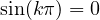 . ∎
The practical consequences: a high-pass filter cannot be made with type II, which is forced to vanish at  ; types III and IV, which vanish at DC, are suited to differentiators and Hilbert transformers, which shift all frequencies by 90°.
The zeros of a linear-phase FIR filter
The symmetry of the coefficients also shows in the  plane:
 . So if
 is a zero, so is
 ; and, since the coefficients are real, so are the conjugates. Zeros come in quadruples
 , or in pairs if they lie on the unit circle or on the real axis. The zeros on the unit circle are the ones that create the dips in the stopband.
Beyond linear phase
If linear phase is not needed, a minimum-phase FIR filter with all its zeros inside the unit circle can be obtained by reflecting the outer ones: it has the same magnitude and a much shorter delay, useful in real-time systems and in control. There is also the frequency sampling method, which fixes the values of the response on a grid of frequencies, and least-squares methods, which minimise the energy of the error instead of its maximum: the ripples are not uniform but the average error is smaller.