The Laplace transform: properties, inversion and stability
Definition and convergence, table of transforms, properties with proof of the derivative rule, initial and final values, partial fractions and the s-plane.
The Fourier transform does not exist for growing signals, such as  , and it does not naturally account for initial conditions. The Laplace transform solves both problems by multiplying the signal by an exponential that damps it. It is the standard tool for circuits in transient conditions and for control engineering: it turns differential equations into algebraic ones and leads directly to the idea of a transfer function.
Definition
For a signal  that is zero for
 (as all signals “switched on” at some instant):

With  you get back the Fourier transform. The real part
 adds a factor
 that damps the signal and makes the integral converge even for exponentially growing functions. The integral converges in the half-plane
 , where
 is the abscissa of convergence.
The basic transforms
Exponential.  , for
 . Every other row of the table follows from this one.
, for  |  |
|---|---|
 |  |
 (step) |  |
 |  |
 |  |
 |  |
 |  |
 | 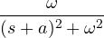 |
 | 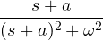 |
Sine and cosine come from  :
 .
Properties
- Linearity.
- Frequency shift:
 . Multiplying by an exponential shifts the transform.
- Delay:
 .
- Derivative:
 , and
 .
- Integral:
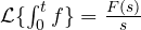 .
- Convolution:
 .
Proof of the derivative rule
Integrating by parts:

because in the half-plane of convergence 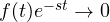 . It is the key property: differentiation becomes multiplication by
 , and the initial conditions enter the equation by themselves. With Fourier you had
 ; here you have , plus the
 term.
Initial and final value theorems

The second holds only if the limit really exists, that is if every pole of  has a negative real part. They give the start and end of a response without inverting: for example the steady-state output of a system after a step.
Inversion with partial fractions
In practical problems is almost always a rational function  . It is split into partial fractions, and each fraction is inverted with the table.
Example.

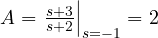 ,
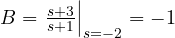 . So
 .
Computing  and
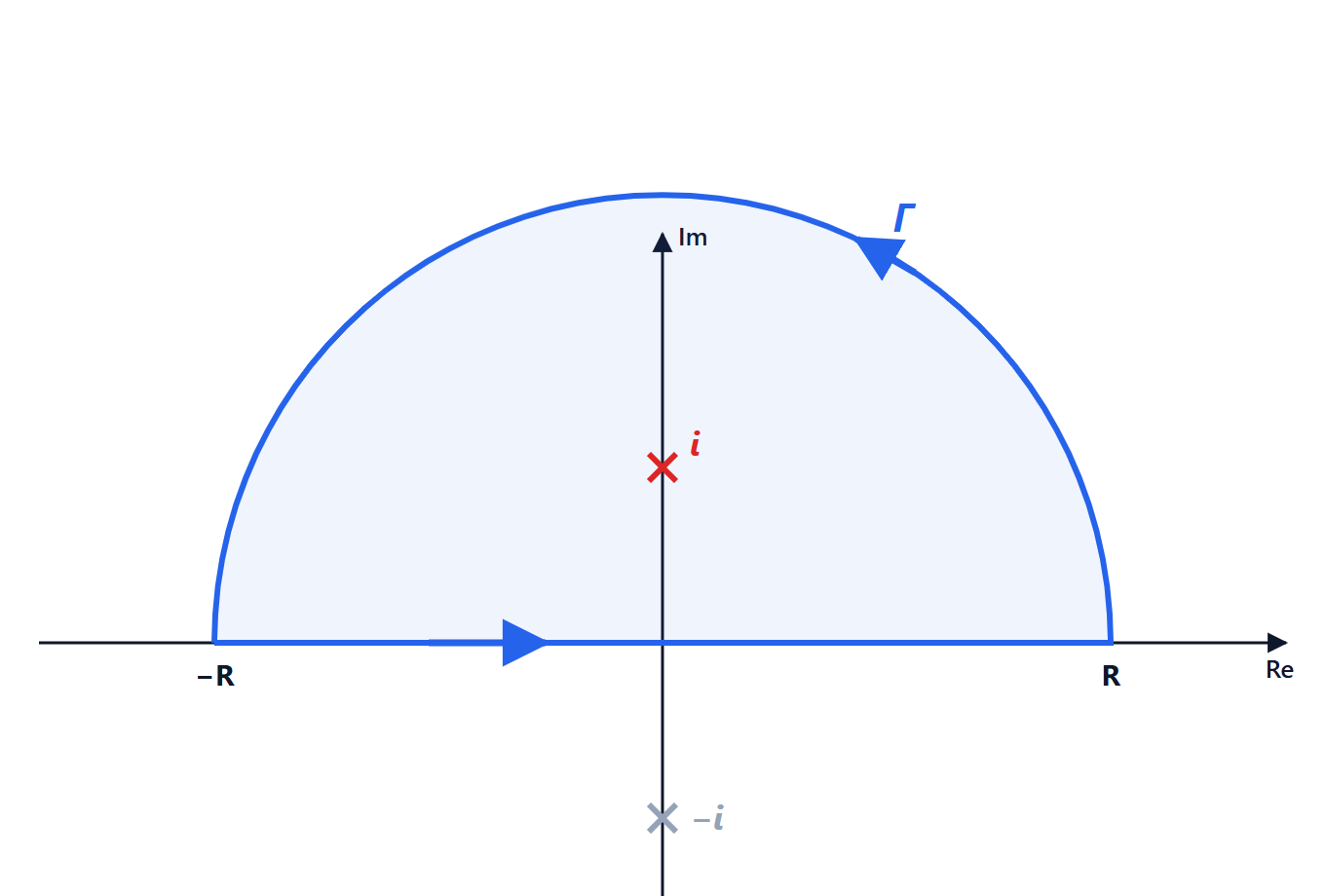
 is exactly the residue computation of the lesson on the residue theorem: in general the inverse transform is the sum of the residues of
 at the poles of
 . A pair of complex conjugate poles
 produces a damped oscillation
 .
The s-plane and stability
Each pole  of contributes to the time response a term
 . The position of the pole in the complex plane therefore tells everything about the behaviour of that term.
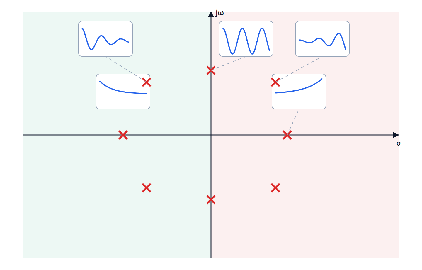
- Negative real part: the term dies away. The further left the pole, the faster.
- Positive real part: the term grows exponentially. The system is unstable.
- On the imaginary axis: an oscillation of constant amplitude (or linear growth if the pole is double).
- The imaginary part gives the frequency of oscillation.
A linear system is stable if and only if every pole of its transfer function has a negative real part. It is the golden rule of control engineering: designing a controller means moving the system’s poles into the right region of the s-plane.