ELECTRONICS ENGINEERINGelectronics-engineering.com

Laplace transform in depth: convergence, properties, final value and inverse transform in every case

Existence and region of convergence, properties proved, initial and final value theorems with the cases where they fail, repeated and complex poles, periodic signals, link with Fourier, tables.

ielettronica 25 October 2026 7 min read 1 comment

https://www.electronics-engineering.com/en/laplace-transform-in-depth-convergence-final-value-inverse/

No ratings yet: be the first to rate this page.

This page goes deeper into the lessons on the Laplace transform and its applications. It proves when the transform exists, derives all the properties in the table, proves the initial and final value theorems together with the cases where they fail, works out the inverse transform with repeated and complex conjugate poles, deals with periodic signals and explains the precise link with the Fourier transform. At the end are the tables to remember.

When the transform exists

A signal $f$ , zero for $t \lt 0$ , is of exponential order if there exist $M$ and $\sigma_0$ with $|f(t)| \le Me^{\sigma_0 t}$ for every $t \ge 0$ . Almost all engineering signals are: polynomials, exponentials, sines, steps. $e^{t^2}$ is not.

Theorem. If $f$ is piecewise continuous and of exponential order $\sigma_0$ , the integral $F(s) = \int_0^\infty f(t)e^{-st}dt$ converges absolutely for $\text{Re}\,s \gt \sigma_0$ , and $F(s) \to 0$ as $\text{Re}\,s \to +\infty$ .

Proof. With $s = \sigma + i\omega$ , $|f(t)e^{-st}| = |f(t)|e^{-\sigma t} \le Me^{-(\sigma - \sigma_0)t}$ , and $\int_0^\infty Me^{-(\sigma - \sigma_0)t}dt = \frac{M}{\sigma - \sigma_0}$ is finite for $\sigma \gt \sigma_0$ . This estimate also gives $|F(s)| \le \frac{M}{\sigma - \sigma_0} \to 0$ . ∎

The half-plane $\text{Re}\,s \gt \sigma_0$ is the region of convergence. For a rational function the boundary passes through the rightmost pole: the transform is analytic (lesson on complex functions) in the whole half-plane, and all the poles lie to the left.

The region of convergence in the s plane — The transform converges in the half-plane to the right of the vertical line sigma zero, shaded in green, which passes through the rightmost pole. All the poles, marked with a cross, lie to the left of that line.

The properties, proved

Shift in s. $\int e^{-at}f(t)e^{-st}dt = \int f(t)e^{-(s + a)t}dt = F(s + a)$ .
Delay. With $u = t - T$ : $\int_T^\infty f(t - T)e^{-st}dt = e^{-sT}\int_0^\infty f(u)e^{-su}du = e^{-sT}F(s)$ .
Second derivative. Applying the derivative rule twice: $\mathcal L\{f''\} = s\mathcal L\{f'\} - f'(0) = s^2F - sf(0) - f'(0)$ .
Integral. If $g(t) = \int_0^t f$ , then $g' = f$ and $g(0) = 0$ : $F = sG$ , i.e. $G = F/s$ .
Multiplication by $t$ . Differentiating the definition with respect to $s$ under the integral sign: $F'(s) = \int(-t)f(t)e^{-st}dt$ , so $\mathcal L\{tf(t)\} = -F'(s)$ . Repeating, $\mathcal L\{t^nf\} = (-1)^nF^{(n)}(s)$ .
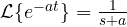
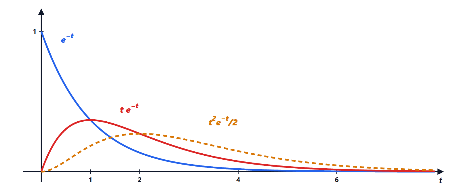
Convolution. $\mathcal L\{f * g\} = \int_0^\infty\int_0^t f(\tau)g(t - \tau)d\tau\,e^{-st}dt$ . Swapping the integrals (integrating over the region $0 \le \tau \le t$ ) and setting $u = t - \tau$ : $\int_0^\infty f(\tau)e^{-s\tau}d\tau\int_0^\infty g(u)e^{-su}du = F(s)G(s)$ .

The rule $\mathcal L\{tf\} = -F'$ explains where the rows of the table with $t^n$ come from: from $\mathcal L\{e^{-at}\} = \frac{1}{s + a}$ one gets $\mathcal L\{te^{-at}\} = \frac{1}{(s + a)^2}$ , $\mathcal L\{t^2e^{-at}\} = \frac{2}{(s + a)^3}$ , and so on. They are the terms produced by repeated poles.

The responses of repeated poles — A simple pole at minus 1 produces e to the minus t; a double pole produces t times e to the minus t, which starts from zero and has a maximum; a triple pole produces t squared times e to the minus t over 2, even slower to start.

The initial and final value theorems

Theorem. If $f$ and $f'$ are transformable, $f(0^+) = \lim_{s\to\infty}sF(s)$ . If moreover all the poles of $sF(s)$ have negative real part, $\lim_{t\to\infty}f(t) = \lim_{s\to 0}sF(s)$ .

Proof. Start from $\int_0^\infty f'(t)e^{-st}dt = sF(s) - f(0^+)$ .

*Initial value:* as $s \to +\infty$ the left-hand side tends to 0 (existence theorem applied to $f'$ ), so $sF(s) \to f(0^+)$ .

*Final value:* as $s \to 0$ the left-hand side tends to $\int_0^\infty f'(t)dt = \lim_{t\to\infty}f(t) - f(0^+)$ , provided this limit exists. So $\lim_{s\to 0}sF(s) = \lim_{t\to\infty}f(t)$ . ∎

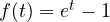When it fails. The final value theorem always gives a number, even when the limit in time does not exist. With $F = \frac{1}{s(s - 1)}$ , $\lim_{s\to 0}sF = -1$ , but $f(t) = e^t - 1$ diverges (the pole at $s = 1$ is on the right). With $F = \frac{1}{s^2 + 1}$ (the sine), $\lim sF = 0$ , but the sine oscillates forever (poles on the imaginary axis). Before using it one must always check the poles.

A case where the final value theorem is wrong — The function e to the t minus 1 diverges, while the formula, applied without checking the poles, would give the value minus 1, dashed.

The inverse transform in every case

For a rational $F = N(s)/D(s)$ with the degree of $N$ less than that of $D$ , the inverse transform is the sum of the residues of $F(s)e^{st}$ at the poles of $F$ (residue theorem applied to the Bromwich integral). In practice:

Simple pole $p$ : contribution $A\,e^{pt}$ , with $A = \lim_{s\to p}(s - p)F(s)$ (Heaviside’s rule: “cover up” the factor $s - p$ and substitute $s = p$ ).

Pole of multiplicity $m$ at $p$ : with $G(s) = (s - p)^mF(s)$ , the contribution is

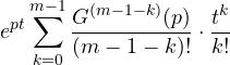
$e^{pt}\sum_{k=0}^{m-1}\frac{G^{(m-1-k)}(p)}{(m - 1 - k)!}\cdot\frac{t^k}{k!}$

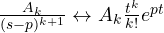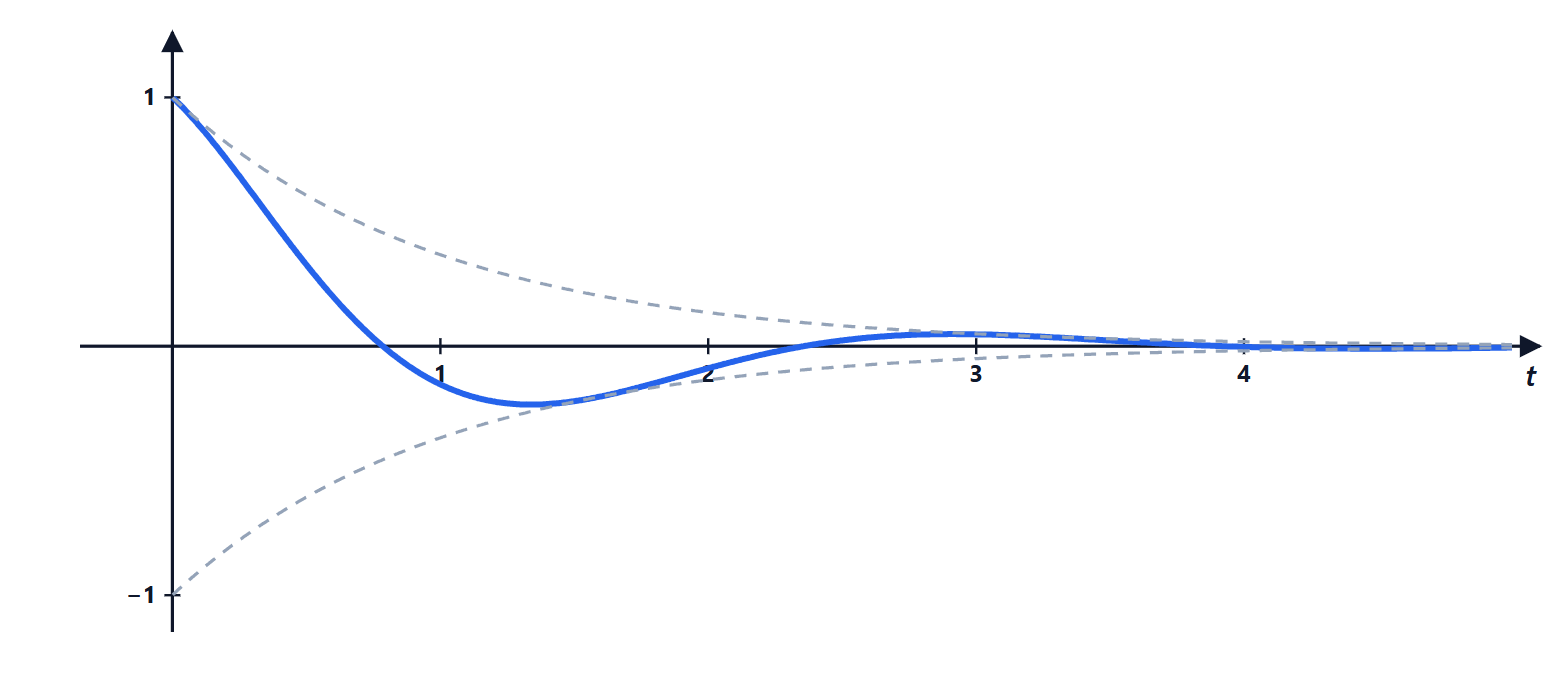
which follows from the fractions $\frac{A_k}{(s - p)^{k+1}} \leftrightarrow A_k\frac{t^k}{k!}e^{pt}$ .

Complex pair $-a \pm ib$ : instead of working with complex numbers, complete the square. A term $\frac{Bs + C}{(s + a)^2 + b^2}$ is rewritten as

$B\,\frac{s + a}{(s + a)^2 + b^2} + \frac{C - Ba}{b}\cdot\frac{b}{(s + a)^2 + b^2} \;\leftrightarrow\; e^{-at}\left(B\cos bt + \frac{C - Ba}{b}\sin bt\right)$

The pair produces an oscillation of angular frequency $b$ inside an envelope $e^{-at}$ : the signature of underdamped second-order systems.

The response of a pair of complex poles — The function e to the minus t times cosine of 2 t oscillates with angular frequency 2 inside the envelope plus and minus e to the minus t, dashed.

Periodic signals

Theorem. If $f$ has period $T$ and $F_1(s) = \int_0^T f(t)e^{-st}dt$ is the transform of the first period, then

$F(s) = \frac{F_1(s)}{1 - e^{-sT}}$

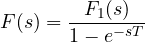
Proof. Split the integral into periods and use the delay: $F = F_1 + e^{-sT}F_1 + e^{-2sT}F_1 + \cdots = F_1\sum_k e^{-ksT}$ , a geometric series with ratio $e^{-sT}$ , with $|e^{-sT}| \lt 1$ for $\text{Re}\,s \gt 0$ . ∎

Example. The square wave that is 1 in the first half of the period and 0 in the second: 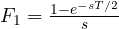$F_1 = \frac{1 - e^{-sT/2}}{s}$ , and $F = \frac{1 - e^{-sT/2}}{s(1 - e^{-sT})} = \frac{1}{s(1 + e^{-sT/2})}$ , because $1 - e^{-sT} = (1 - e^{-sT/2})(1 + e^{-sT/2})$ . There are infinitely many poles, on the imaginary axis, corresponding to the harmonics of the Fourier series.

Periodic square wave — The wave is 1 in the first half of each period and 0 in the second; its transform is obtained from that of the first period.

The link with Fourier

If the region of convergence contains the imaginary axis (i.e. $\sigma_0 \lt 0$ : all poles on the left), then the Fourier transform of the causal signal exists and equals $F(i\omega)$ . For a stable system, therefore, the frequency response is obtained by substituting $s = i\omega$ in the transfer function. If instead there are poles on the axis (step, sine) the Fourier transform exists only as a distribution and contains deltas; if there are poles on the right it does not exist at all, while Laplace does: this is why control theory uses Laplace, which also handles unstable systems that need to be stabilised.

Tables to remember

Transforms (for $t \ge 0$ )

$f(t)$	$F(s)$
$\delta(t)$	1
$u(t)$	$\dfrac{1}{s}$
$t^n$	$\dfrac{n!}{s^{n+1}}$
$e^{-at}$	$\dfrac{1}{s + a}$
$t^ne^{-at}$	$\dfrac{n!}{(s + a)^{n+1}}$
$\sin bt$ , $\cos bt$	$\dfrac{b}{s^2 + b^2}$ , $\dfrac{s}{s^2 + b^2}$
$e^{-at}\sin bt$ , $e^{-at}\cos bt$	$\dfrac{b}{(s + a)^2 + b^2}$ , $\dfrac{s + a}{(s + a)^2 + b^2}$
$\sinh bt$ , $\cosh bt$	$\dfrac{b}{s^2 - b^2}$ , $\dfrac{s}{s^2 - b^2}$
$t\sin bt$	$\dfrac{2bs}{(s^2 + b^2)^2}$
$\dfrac{\sin bt - bt\cos bt}{2b^3}$	$\dfrac{1}{(s^2 + b^2)^2}$
$1 - e^{-at}$	$\dfrac{a}{s(s + a)}$

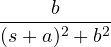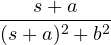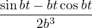Properties

Time	Laplace
$e^{-at}f(t)$	$F(s + a)$
$f(t - T)u(t - T)$	$e^{-sT}F(s)$
$f(at)$ , $a \gt 0$	$\frac{1}{a}F(s/a)$
$f'(t)$	$sF(s) - f(0)$
$f''(t)$	$s^2F(s) - sf(0) - f'(0)$
$\int_0^t f$	$F(s)/s$
$tf(t)$	$-F'(s)$
$f(t)/t$	$\int_s^\infty F(\sigma)\,d\sigma$
$f * g$	$F(s)G(s)$
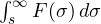periodic with period $T$	$F_1(s)/(1 - e^{-sT})$

Second-order system $G(s) = \frac{\omega_n^2}{s^2 + 2\zeta\omega_ns + \omega_n^2}$ , with $0 \lt \zeta \lt 1$ : overshoot $M_p = e^{-\pi\zeta/\sqrt{1 - \zeta^2}}$ ; peak time 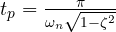$t_p = \frac{\pi}{\omega_n\sqrt{1 - \zeta^2}}$ ; 2 % settling time $t_s \approx \frac{4}{\zeta\omega_n}$ ; damped angular frequency $\omega_d = \omega_n\sqrt{1 - \zeta^2}$ .

Exercises from basic to exam level, with differential equations, circuits and systems, are on the exercise page linked at the top.

1 Comment

Oldest

Newest Most Voted

Author

ielettronica

9 hours ago

Sono l'autore di questa pagina su «Trasformata di Laplace, approfondimento: convergenza, proprietà, valore finale e antitrasformata in tutti i casi». Se qualcosa non è chiaro, se vi serve un esempio in più o volete approfondire un punto, scrivetelo qui sotto nei commenti: rispondo personalmente. Se la pagina vi è stata utile, lasciate un voto con le stelle in cima all'articolo.I am the author of this page on “Laplace transform in depth: convergence, properties, final value and inverse transform in every case”. If something is unclear, if you need another example or want to go deeper into a point, write it in the comments below: I answer personally. If the page was useful, leave a star rating at the top of the article.

Cookie	Duration	Description
cookielawinfo-checkbox-analytics	11 months	This cookie is set by GDPR Cookie Consent plugin. The cookie is used to store the user consent for the cookies in the category "Analytics".
cookielawinfo-checkbox-functional	11 months	The cookie is set by GDPR cookie consent to record the user consent for the cookies in the category "Functional".
cookielawinfo-checkbox-necessary	11 months	This cookie is set by GDPR Cookie Consent plugin. The cookies is used to store the user consent for the cookies in the category "Necessary".
cookielawinfo-checkbox-others	11 months	This cookie is set by GDPR Cookie Consent plugin. The cookie is used to store the user consent for the cookies in the category "Other.
cookielawinfo-checkbox-performance	11 months	This cookie is set by GDPR Cookie Consent plugin. The cookie is used to store the user consent for the cookies in the category "Performance".
viewed_cookie_policy	11 months	The cookie is set by the GDPR Cookie Consent plugin and is used to store whether or not user has consented to the use of cookies. It does not store any personal data.

When the transform exists

The properties, proved

The initial and final value theorems

The inverse transform in every case

Periodic signals

The link with Fourier

Tables to remember

Related articles

From imitation to reinforcement learning: how Chinese driving systems are trained

BJT logic gates: RTL, DTL, TTL 7400, Schottky and ECL

Navigate on Autopilot in China: how city NOA became a mass-market feature

The chips and sensors behind China’s assisted driving

Z transform in depth: stability, z plane, ZOH, Euler and Tustin

Anisotropic media: the Polder tensor of ferrite, birefringent crystals, ionospheric plasma and the Hall effect