Laplace in practice: differential equations, circuits and the transfer function
Solving differential equations, impedances in the s domain, the transfer function and feedback, the second-order system, overshoot and settling time.
With the Laplace transform a differential equation with its initial conditions becomes an algebraic equation, solved with basic arithmetic. In this lesson we use it to solve differential equations, to analyse circuits directly in the  domain and to study the transfer function and the step response of second-order systems, the most common in electronics and control.
Solving a differential equation
The method has three steps: transform the equation, solve for  , invert.
Example.

Transforming, with  and
 :

Partial fractions: 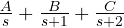 , with
 ,
 ,
 . So

Check:  ,
 , and in steady state
 , as the final value theorem says:
 . No constants to find at the end: the initial conditions entered the calculation from the start.
Circuits in the s domain
Transforming the component laws, with zero initial conditions:
| Component | Time | domain | Impedance |
|---|---|---|---|
| resistor |  |  |  |
| inductor |  |  |  |
| capacitor | 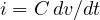 |  |  |
They are the impedances of the AC lesson with in place of  . The circuit is solved with the generalised Ohm’s law, dividers and Kirchhoff’s laws, as if it were made of resistors. Non-zero initial conditions are represented by extra sources: a capacitor charged to
 becomes the impedance
 in series with a source
 .
Example: the RC low-pass. The divider between and gives

With a step input,  , one gets
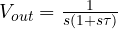 and therefore
 : the capacitor charging, in three lines.
The transfer function
For a linear system with zero initial conditions, the ratio of the output and input transforms does not depend on the input:
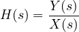
It is the transfer function, and it is the Laplace transform of the impulse response. It holds the whole system:
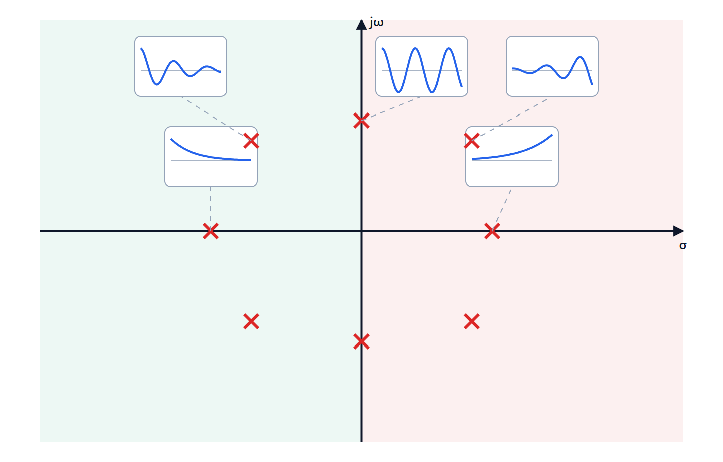
- its poles give the natural modes and stability;
- evaluated at
 it gives the frequency response:
 is the gain and
 the phase shift at each frequency, from which Bode plots are drawn;
- multiplied by the input transform it gives the output.
Cascading systems means multiplying transfer functions. With negative feedback, a block  with feedback
 becomes
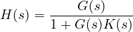
the formula behind feedback op-amp amplifiers and every control system.
The second-order system
A great many systems (the RLC circuit, a suspension, a hard disk motor) behave like
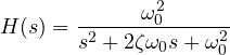
where  is the natural angular frequency and
 the damping ratio. The poles are

real and distinct if  , coincident if
 , complex conjugate if
 .
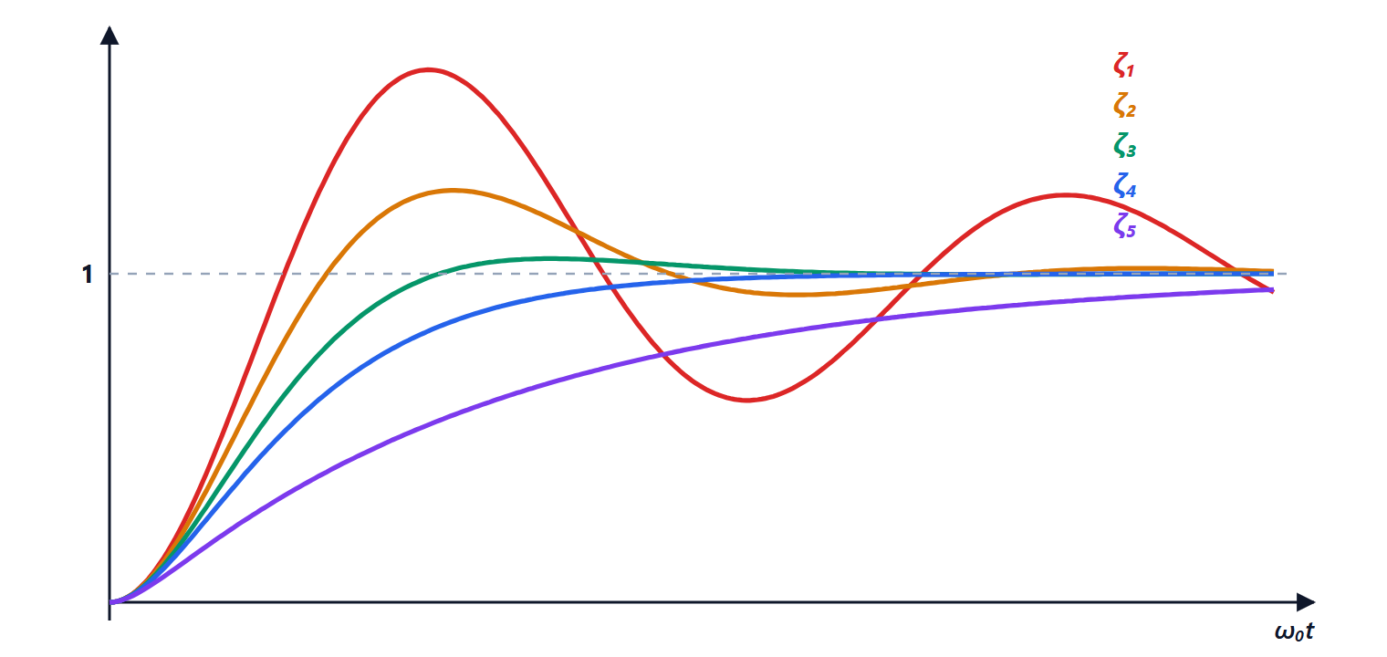
 ,
 ,
 ,
 and
 . With low damping the response overshoots the final value and rings for a long time; with it arrives without overshooting; with high damping it is slow.
For the step response is

The parameters found in specifications:
- the maximum overshoot,
 : 37% with
 , 4.6% with
 , zero with
 ;
- the 2% settling time, about
 ;
- the rise time, inversely proportional to .
The value  is a classic compromise: a fast response with an overshoot of a few per cent. It is the damping of a second-order Butterworth filter (
 ), the one with the flattest possible frequency response.
Example. A series RLC with the output across the capacitor has  , so
 and
 . With
 mH and
 µF,
 rad/s (5 kHz); to get you need
 Ω.