Stability and the Routh-Hurwitz criterion
Stability and pole locations, the necessary condition on coefficients with proof, the Routh table, the third-degree case, maximum gain and oscillation at the limit.
The first requirement of any control system is stability: after a disturbance it must return to normal operation, not oscillate more and more or diverge. A badly designed feedback loop can make even a perfectly stable plant unstable. In this lesson we cover the link between stability and pole locations and the Routh-Hurwitz criterion, which establishes stability without computing the roots.
Stability and poles
For a linear system with a rational transfer function, the impulse response is a sum of terms  , one for each pole
 (with
 up to the multiplicity minus one). It follows that:
- if all poles have negative real part, every term tends to zero, the impulse response is absolutely integrable and the system is stable (BIBO, as in the Signal Theory lesson);
- if even one pole has positive real part, the corresponding term grows without bound: unstable;
- simple poles on the imaginary axis give constant terms or sustained oscillations: the system is on the edge (marginally stable), and an input at the same frequency makes it diverge.
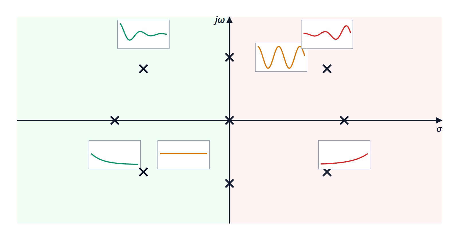
The stability of a closed loop therefore depends on the roots of  , the characteristic equation. For a high-degree polynomial the roots cannot be computed by hand, but to know whether a system is stable it is enough to know the sign of their real parts.
A necessary condition
Theorem. If all roots of a real polynomial  , with
 , have negative real part, then all coefficients are positive.
Proof. The polynomial is  times the product of factors
 for the real roots
 , with
 , and
 for the complex pairs
 . All these factors have positive coefficients, and the product of polynomials with positive coefficients has positive coefficients. ∎
A zero or negative coefficient is therefore enough to say the system is not stable. The converse does not hold:  has all positive coefficients but two roots with positive real part.
The Routh-Hurwitz criterion
A table is built. The first two rows contain the coefficients of the polynomial, alternating:
 | |  |  | … |
|---|---|---|---|---|
 |  |  |  | … |
 |  |  | … |
and each new row is computed from the two above with

down to the  row.
Criterion (statement). The number of roots with positive real part equals the number of sign changes in the first column. The system is stable if and only if all elements of the first column have the same sign.
The third-degree case. For  the first column is
 : the system is stable if and only if all coefficients are positive and

In the example :  , unstable, as stated.
The maximum gain
The typical use is finding the range of gain that keeps the loop stable.
Example. Plant  with a proportional controller
 . The characteristic equation is

By the third-degree criterion:  and
 . The loop is stable for
 . At the limit,
 , the
 row vanishes and the
 row gives the auxiliary equation
 , that is
 : the system oscillates at
 rad/s. We will meet this again in the lesson on the root locus.
This example shows the general behaviour: with a low gain the system is stable but slow and inaccurate; increasing it makes it quicker, then less and less damped, and beyond a limit unstable. Controller design is the search for the best compromise within these limits.