The Nyquist criterion and stability margins
The critical point −1, the Nyquist criterion and the argument principle, an example with plot, gain and phase margins on Bode plots, link with damping, delays.
The Routh criterion and the root locus need a model of the plant as a rational function. Often, however, the plant is known through its frequency response, measured with an analyser or obtained from tests, and the plant may contain pure delays that are not rational. The Nyquist criterion decides closed-loop stability by looking only at the open-loop frequency response, and in addition gives a measure of how far the system is from instability: the gain and phase margins.
The idea
The closed loop is unstable if  has roots in the right half-plane. The critical point is
 : if at some frequency the loop function equals exactly −1, the signal going round the loop comes back identical (gain 1, 180° phase shift, which with the minus sign of the comparison becomes 360°) and the system oscillates on its own. It is the same principle as an electronic oscillator, and as the howl of a microphone held too close to its loudspeaker.
The Nyquist criterion
The Nyquist plot is the curve traced in the complex plane by  as
 goes from
 to
 (the part for
 is the mirror image about the real axis).
Criterion (statement). Let  be the number of poles of
 in the right half-plane and
 the number of times the Nyquist plot encircles the point −1, counted positive clockwise. The number of closed-loop poles in the right half-plane is

The closed loop is stable if and only if  .
Where it comes from. It is an application of the argument principle, a consequence of the residue theorem (Mathematical Methods lessons): as  travels along a closed curve enclosing the whole right half-plane, the image
 winds around the origin a number of times equal to the difference between the zeros and poles of
 enclosed. The zeros of are the closed-loop poles, its poles are those of
 ; and winding around the origin for is the same as winding around −1 for . (If has poles on the imaginary axis, like integrators, the curve goes around them with small semicircles.)
The common case. If is stable ( ), the closed loop is stable if and only if the plot does not encircle the point −1.
An example
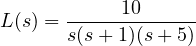
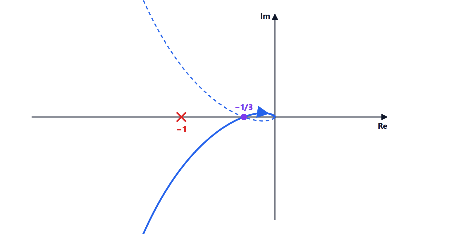
The plot crosses the negative real axis where the phase is −180°:  rad/s, with
 . The point −1 stays outside: the closed loop is stable. Multiplying the gain by 3 would make the curve pass exactly through −1: the same limit
 given by the Routh criterion on the equation
 (
 ).
Stability margins
The further the curve passes from −1, the more robust the system. The distance is measured by two numbers, which can also be read conveniently on the Bode plots of :
- gain margin
 : by how much the gain can be multiplied before instability,
 , where
 is the frequency at which the phase is −180°;
- phase margin
 : how much extra phase lag can be added before instability,
 , where
 is the crossover frequency at which
 (0 dB).
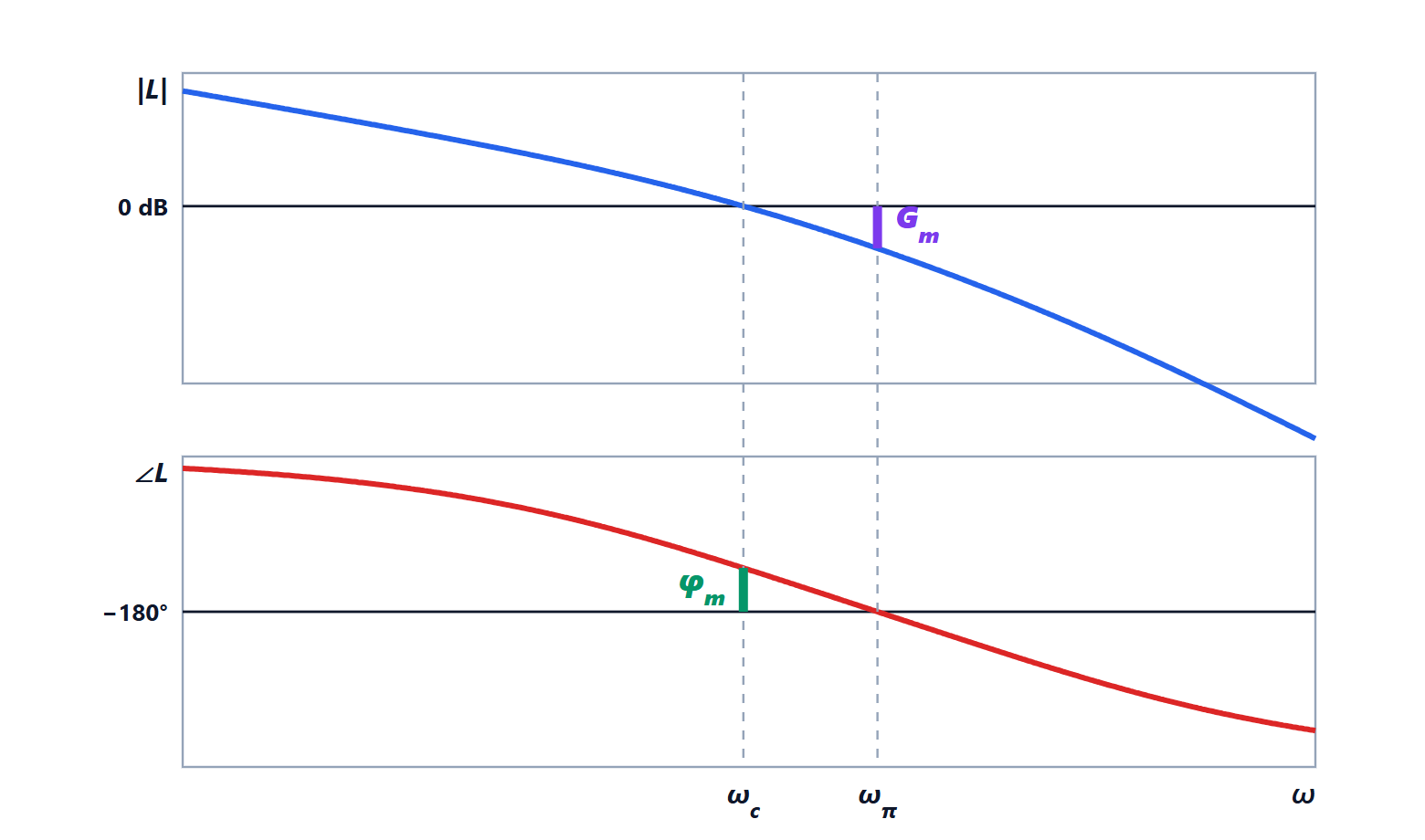
In the example:  , that is 9.5 dB, and
 rad/s with
 .
Phase margin and damping. For a loop that behaves like a second-order system,  holds to a good approximation (with in degrees, up to about 60°). A 25° margin means
 and an overshoot around 44% (simulating the closed loop gives 49%): stable, but too oscillatory. In practice phase margins of 45 to 60° and gain margins of at least 6 dB are required. In the lesson on compensators we will increase the margin of this example.
Delays. A pure delay  (transport time on a conveyor belt, network latency) has magnitude 1 and phase
 : it does not change the magnitude plot, but it takes away phase margin increasingly with frequency. The Nyquist criterion handles it with no difficulty, which is one reason frequency-domain design is so widely used in industry.