Bode plots and the Nyquist criterion in depth: rules, resonance, criterion proved and margins
Bode plot asymptotes and errors, second-order resonance proved, minimum phase, delays and unstable zeros, argument principle and Nyquist criterion proved, gain, phase and delay margins, MATLAB and Python examples.
This page goes deeper into the lesson on the Nyquist criterion and stability margins. It derives the rules for drawing Bode plots by hand (asymptotes, errors, second-order resonance, delays, non-minimum-phase zeros), proves the Nyquist criterion from the argument principle, explains how to deal with an integrator or an open-loop unstable process, and links gain, phase and delay margins to performance. At the end are the examples in MATLAB and Python, with verified code.
Why Bode plots are drawn by adding
A rational transfer function can be written as a product of elementary factors:

With  , the logarithm turns the product into a sum:
 and
 . So it is enough to know the plots of the elementary factors and add them.
The simple pole  : magnitude
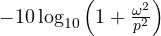 dB.
- For
 it is about 0 dB; for
 it is
 : a straight line with slope −20 dB per decade that crosses 0 dB at
 . The two lines are the asymptotes.
- The largest error is at the corner:
 dB. One octave away (
 or
 ) the error is
 dB.
- The phase
 is
 at and goes from 0 to
 ; the piecewise approximation makes it fall linearly between
 and
 , with a maximum error of about 5.7°.
The zero gives the same plots with the opposite sign; the integrator  is a line at −20 dB per decade at all frequencies, with constant phase .
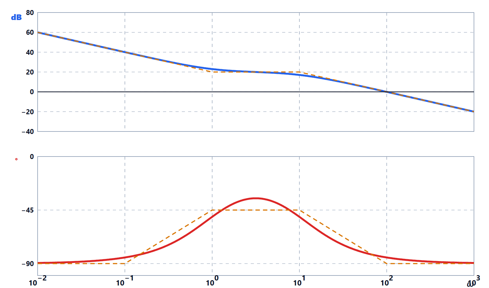
Second-order resonance
Theorem. The system  , with
 , has a resonant peak at
 , of height
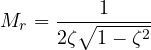
For  the magnitude is decreasing and there is no peak.
Proof. With  :
 . Look for the minimum of this function of
 :
 ,
 ,
 , acceptable only if positive. There
 , and
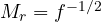 . ∎
With  the peak is
 , i.e. 14 dB; with
 , 8.1 dB; with
 , 2.7 dB. At
 the phase is always . The asymptote error (the asymptote has a corner at 0 dB at
 and then falls by 40 dB per decade) can be large: for lightly damped systems Bode cannot be drawn with straight lines alone.

Minimum phase, delays, unstable zeros
A system with no poles or zeros in the right half-plane and no delays is called minimum phase. For these systems the phase is determined by the magnitude (Bode’s gain-phase relation): where the magnitude falls with a constant slope of  dB per decade, the phase approaches
 degrees. This is why, in design, one tries to cross 0 dB with a slope of −20 dB per decade: the phase is then around , far from
 .
Two important exceptions:
- a delay
 has magnitude 1 and phase
 (in radians), which grows without limit: it does not change the magnitude but removes phase margin, the more so the higher the crossover frequency;
- a zero in the right half-plane, like
 , has the same magnitude as the stable zero but a phase that falls instead of rising. The system
 has magnitude 1 at all frequencies and phase from 0 to . In time, an unstable zero makes the step response start in the wrong direction (undershoot): this happens in boost converters, in aircraft pitch dynamics, in the drum level of a boiler.
The Nyquist criterion, proved
Argument principle. Let  be a rational function and
 a closed curve, traversed clockwise, that does not pass through zeros or poles of
 . If inside there are
 zeros and
 poles of (counted with multiplicity), the image curve
 goes round the origin
 times clockwise.
Proof. Writing  , we have
 . When
 goes once round clockwise, the vector
 rotates by
 if
 is inside the curve and returns to the same angle (zero change) if it is outside. So the total change in the argument of is
 : clockwise turns. In integral form it is
 (with the curve traversed anticlockwise), a direct consequence of the residue theorem, because
 has residue
 at each simple zero and
 at each simple pole. ∎
The criterion. Apply the principle to  , with the Nyquist contour: the imaginary axis from
 to
 and a semicircle of radius
 in the right half-plane, which therefore encloses the whole right half-plane. The zeros of
 are the closed-loop poles; the poles of are those of
 . Going round the origin with is the same as going round with . On the large semicircle
 (proper systems), and the image shrinks to a point: it is enough to draw
 . This gives

with  the clockwise turns round , the poles of in the right half-plane, the closed-loop poles in the right half-plane. ∎
Poles on the imaginary axis. If has poles on the axis (for example an integrator at 0), the contour goes round them with small semicircles of radius  to the right, leaving them outside. For a simple pole at 0,
 and on
 , with
 from to
 , the image is
 : a semicircle of infinite radius traversed clockwise, which closes the plot “from infinity”.

Margins and robustness
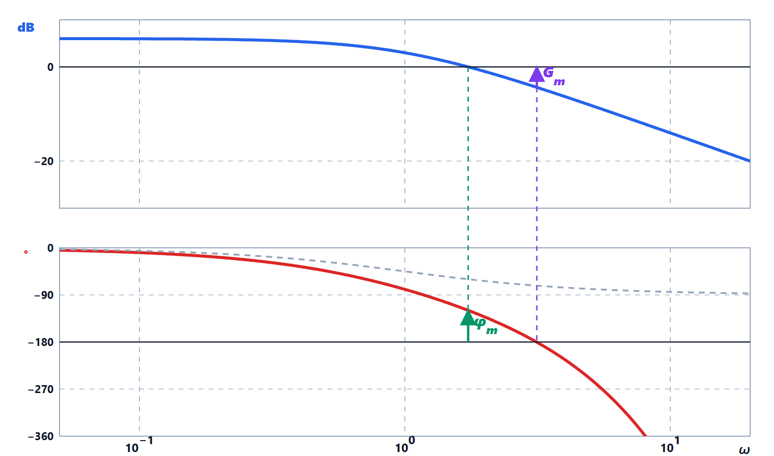
With  the crossover frequency (
 ) and
 the frequency where the phase is :
- gain margin
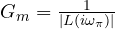 : the factor by which the gain can be multiplied before instability;
- phase margin
 : the extra phase lag that can be tolerated;
- delay margin
 (with
 in radians): the pure delay that would cause instability. It is the most meaningful margin in systems controlled by a processor or through a network;
- sensitivity peak
 : the inverse of the minimum distance of the Nyquist plot from . Typical design values:
 (6 dB), which guarantees
 and
 .
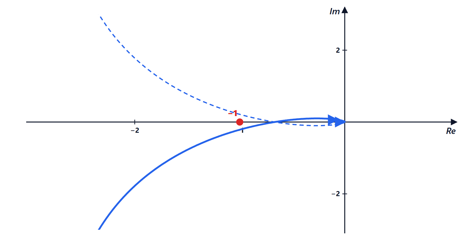
Example. For  :
 ,
 ,
 (3.5 dB);
 rad/s,
 , delay margin 0.17 s. The system is stable but fragile: the step response has an overshoot of 70 %.

Bode and Nyquist in MATLAB and Python
MATLAB:
L = tf(4, [1 3 2 0]);           % L(s) = 4/(s(s+1)(s+2))
margin(L)                        % Bode with the margins written on the plot
[Gm, Pm, Wpc, Wgc] = margin(L)
nyquist(L)
step(feedback(L, 1))
Python (numpy and python-control):
import numpy as np
import control as ct

L = ct.tf([4], [1, 3, 2, 0])            # L(s) = 4/(s(s+1)(s+2))
gm, pm, wpc, wgc = ct.margin(L)
print(f"Gm = {gm:.2f} ({20*np.log10(gm):.1f} dB) at {wpc:.3f} rad/s")
print(f"PM = {pm:.1f} degrees at {wgc:.3f} rad/s")
print(f"delay margin = {np.radians(pm)/wgc:.3f} s")
T = ct.feedback(L, 1)
print(f"overshoot = {ct.step_info(T)['Overshoot']:.0f} %")
Running it prints  (3.5 dB) at 1.414 rad/s, at 1.143 rad/s, delay margin 0.174 s and overshoot 70 %. The plots are obtained with
ct.bode_plot(L, dB=True, margins=True) and ct.nyquist_plot(L), which use matplotlib.
Exercises with hand-drawn plots, margins, delays and open-loop unstable systems are on the exercise page linked at the top.